Appendix J — Solving Initial-Value ODEs

This appendix examines the numerical solution of sets of initial value ordinary differential equations (IVODEs). There are many software packages that include an IVODE solver (a function that can be used to solve sets of IVODEs). Under the assumption that different readers will choose to use different software packages, the discussion in this appendix is general. Nonetheless it provides sufficient information for readers to follow Reaction Engineering Basics examples wherein sets of IVODEs ae solved, and to implement them using the IVODE solver they prefer. Of course it will be necessary to consult the documentation for the chosen solver to learn the details for using it. Readers seeking a more complete understanding of how IVODE solvers work should consult a numerical methods textbook or take a course on numerical methods.

J.1 Identifying IVODEs

A differential equation contains at least one derivative. A distinguishing feature of a set of ordinary differential equations is that every derivative that appears in the equations has the same independent variable. Put differently, there are no partial derivatives in a set of ordinary differential equations. In virtually all cases, the sets of IVODEs that are solved in Reaction Engineering Basics are linear, first-order ODEs. That means that there are no higher order derivatives in the equations and that there are no products, quotients or powers of the first-order derivatives.

Thus, the sets of IVODEs under consideration here will take the form shown in Equations J.1 through J.4. In those equations \(x\) is the independent variable; \(y_1\), \(y_2\), \(y_3\), and \(y_4\) are the dependent variables; and \(m_{1,1}\) through \(m_{4,4}\) and \(g_1\) through \(g_4\) can be constants or functions of the independent and dependent variables.

\[ m_{1,1}\frac{dy_1}{dx} + m_{1,2}\frac{dy_2}{dx} + m_{1,3}\frac{dy_3}{dx} + m_{1,4}\frac{dy_4}{dx} = g_1 \tag{J.1}\]

\[ m_{2,1}\frac{dy_1}{dx} + m_{2,2}\frac{dy_2}{dx} + m_{2,3}\frac{dy_3}{dx} + m_{2,4}\frac{dy_4}{dx} = g_2 \tag{J.2}\]

\[ m_{3,1}\frac{dy_1}{dx} + m_{3,2}\frac{dy_2}{dx} + m_{3,3}\frac{dy_3}{dx} + m_{3,4}\frac{dy_4}{dx} = g_3 \tag{J.3}\]

\[ m_{4,1}\frac{dy_1}{dx} + m_{4,2}\frac{dy_2}{dx} + m_{4,3}\frac{dy_3}{dx} + m_{4,4}\frac{dy_4}{dx} = g_4 \tag{J.4}\]

While four equations are being used here for illustration purposes, there can be any number of ordinary differential equations in the set as long as the number of ordinary differential equations is equal to the number of dependent variables, and there is only one independent variable. In Reaction Engineering Basics, the independent variable is either the elapsed time, \(t\), or the axial position, \(z\), measured from the inlet of a plug flow reactor.

Numerical solution finds the values of the independent and dependent variables over a continuous range. The values of the independent and dependent variables at the start of that range are called their initial values, and the values of the independent and dependent variables at the end of the range are called their final values.

J.2 IVODE Solvers

The inner workings of IVODE solvers are beyond the scope of Reaction Engineering Basics. Nonetheless, a simplified understanding of how IVODEs are solved numerically is useful. When an IVODE solver is called, it must be provided with the following arguments: the initial values, the stopping criterion (i. e. the final value of either the independent variable or one of the dependent variables), and a derivatives function. As described below, the derivatives function uses the IVODEs to calculate and return the values of the derivatives appearing in the IVODEs.

The solver starts from the initial values, as illustrated graphically in part (a) of Figure J.1 for any one of the dependent variables. It isn’t possible to plot \(y\) vs. \(x\) at that point because \(y\left(x\right)\) is not known. (Indeed, \(y\left(x\right)\) is the solution to the IVODE.) Instead, the solver uses the IVODEs to calculate the value of each of the derivatives at \(\left(x_0,y_0\right)\). The derivative, \(\frac{dy}{dx}\), at that point is the slope of the unknown function at \(\left(x_0,y_0\right)\). This is shown graphically in part (b) of Figure J.1.

Figure J.1: Graphical Representation of an IVODE Integration Step. (a) The initial value. (b) The slope at that point. (c) Incrementally increasing x and approximating the corresponding y.

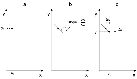
Starting from the known point, \(\left(x_0,y_0\right)\), the solver increases \(x\) by a small amount, \(\Delta x\), which is known as the step-size. It then calculates the corresponding change in \(y\), \(\Delta y\), using the slope. The resulting point, \(\left(x_1,y_1\right)\), is shown in part (c) of Figure J.1. This process is sometimes referred to as taking an integration step. Effectively, the solver uses the small straight line segment between \(\left(x_0,y_0\right)\) and \(\left(x_1,y_1\right)\) to approximate the true solution, \(y\left(x\right)\), in that interval. The accuracy of this approximation increases as \(\Delta x\) decreases, so typically the solver uses small steps. A new integration step is then taken starting fr0m \(\left(x_1,y_1\right)\).

Of course, the solver eventually must stop taking integration steps. After completing each step, the solver checks to determine whether making that step resulted in the stopping criterion being satisfied. If not, the solver takes another integration step. As an example, suppose the stopping criterion is that \(y_3\) should equal some value, \(y_{3,f}\), the solver would check to see whether \(y_3\) did, in fact, reach or surpass \(y_{3,f}\) after making the step. In most cases the stopping criterion will have been surpassed by some small amount, in which case the solver interpolates to find final values that exactly satisfy the stopping criterion. It then returns the values of the dependent variables and the independent variable for all of the steps it took while solving the IVODEs, including those final interpolated values.

J.2.1 Cautions Related to Numerical Solution of IVODEs

When the stopping criterion is a value of one of the dependent variables, many solvers require that you provide both a final value of the independent variable and the known final value of that dependent variable. The solver then takes steps as described above, and after each step it checks to see whether either variable has reached its specified final value. The problem is that if you specify a final value of the independent variable that is too small, the solver may reach that value first and stop. The stopping criterion you specified for the dependent variable will not have been reached, and the result that is returned is not the result you are seeking. Therefore it is important to check that the dependent variable reached the specified final value.

To avoid having the solver stop because it reached the stopping criterion for the independent variable, it is tempting to specify a very large final value for the independent variable stopping criterion. The problem with doing this is that it may cause the solver to use a step size that is too large, resulting in an inaccurate solution. Therefore, it is important to check that the step size was not too large. The solution that is returned will include the final value of the independent variable. The stopping criterion for the independent variable can be set to a value slightly larger than that and the equations can be solved a second time. Assuming the second solution reaches the desired stopping criterion for the dependent variable, the second solution should be accurate.

A second possible problem arises when solving sets of IVODEs where one of the dependent variables changes very abruptly over a very small range of the independent variable. The abrupt changes in that dependent variable may significantly affect the other dependent variables over a much broader range of the independent variable. Equations like this are called stiff ODEs, and they require special treatment of the step size. Therefore, when solving sets of ODEs, one should pay attention to whether any of the dependent variables change very abruptly as the independent variable changes. If they do, it is advisable to repeat the solution using a solver that is specifically tailored to stiff ODEs.

J.3 Input Required by IVODE Solvers

The preceeding discussion shows that IVODE solvers need three things in order to solve a set of IVODEs. The first are the initial values from which the solver will take the first integration step. The second is the name of a function, written by the reaction engineer, that the solver can use to evaluate the derivatives, that is to calculate the numerical values of the derivatives. Herein, this function will be referred to as the derivatives function. The third required input to an IVODE solver is a stopping criterion that the solver can use to decide when to stop taking integration steps. As noted above, a stopping criterion has two parts: the identity of the variable (the independent variable or one of the dependent variables) and its final value.

J.3.1 Derivative Expressions and the Derivatives Function

It was noted above that one input required by an IVODE solver is the name of a function, written by the reaction engineer, that the solver can use to evaluate the derivatives. More specifically, the derivatives function must accept the independent variable and the dependent variables corresponding to the start of an integration step as input arguments, and it must use them to calculate and return the values of the derivatives that appear in the IVODEs.

To do so, it is useful to convert the IVODEs into a set of expressions for the individual derivatives if they aren’t already in that form. For example, Equations J.1 through J.4 need to be converted to derivative expressions of the form shown in Equations J.5 through J.8 where \(f_1\), \(f_2\), \(f_3\), and \(f_4\) each may be a function of \(x\), \(y_1\), \(y_2\), \(y_3\), and \(y_4\).

\[ \frac{dy_1}{dx} = f_1 \tag{J.5}\]

\[ \frac{dy_2}{dx} = f_2 \tag{J.6}\]

\[ \frac{dy_3}{dx} = f_3 \tag{J.7}\]

\[ \frac{dy_4}{dx} = f_4 \tag{J.8}\]

That can be accomplished by algebraic manipulation of Equations J.1 through J.4, but it is particularly straightforward if the original IVODEs are written as a matrix equation. The coefficients in Equations J.1 through J.4, \(m_{1,1}\), \(m_{1,2}\), etc., can be used to construct a so-called mass matrix, \(\boldsymbol{M}\), as shown in Equation J.9, the dependent variables can be used to construct a column vector, \(\underline{y}\), as in equation Equation J.10, and the functions, \(g_1\), \(g_2\), \(g_3\), and \(g_4\), can be used to construct a column vector, \(\underline{g}\), as in equation Equation J.11.

\[ \boldsymbol{M} = \begin{bmatrix} m_{1,1} \ m_{1,2} \ m_{1,3} \ m_{1,4} \\m_{2,1} \ m_{2,2} \ m_{2,3} \ m_{2,4} \\m_{3,1} \ m_{3,2} \ m_{3,3} \ m_{3,4} \\ m_{4,1} \ m_{4,2} \ m_{4,3} \ m_{4,4} \end{bmatrix} \tag{J.9}\]

\[ \underline{y} = \begin{bmatrix} y_1 \\ y_2 \\ y_3 \\ y_4 \end{bmatrix} \tag{J.10}\]

\[ \underline{g} = \begin{bmatrix} g_1 \\ g_2 \\ g_3 \\ g_4 \end{bmatrix} \tag{J.11}\]

Equations J.1 through J.4 then can be written as a matrix equation, Equation J.12. Pre-multiplying each side of Equation J.12 by the inverse of the mass matrix yields the desired derivative expressions, Equation J.13. That is, comparing Equation J.13 to Equations J.5 through J.8, it is apparent that they are equivalent with \(f_1\), \(f_2\), \(f_3\), and \(f_4\) given by Equation J.14.

\[ \boldsymbol{M}\frac{d}{dx}\underline{y} = \underline{g} \tag{J.12}\]

\[ \frac{d}{dx}\underline{y} = \boldsymbol{M}^{-1} \underline{g} \tag{J.13}\]

\[ \begin{bmatrix} f_1 \\ f_2 \\ f_3 \\ f_4 \end{bmatrix} = \underline{f} = \boldsymbol{M}^{-1} \underline{g} \tag{J.14}\]

Wring the IVODEs in the form of derivatives expressions, facilitates evaluating the derivatives. The derivatives function will be provided with the independent and dependent variables as arguments. They can be used, along with known constants provided as part of the assignment, to evaluate each of the \(f\) functions in Equations J.5 through J.8, or equivalently in Equation J.14.

The \(f\) functions may also contain other variables and possibly, an unknown constant. The other variables clearly must be calculated in order to evaluate the \(f\) functions. This is done using expressions for those other variables in terms of known constants and the independent and dependent variables.

If the \(f\) functions contain an unknown constant, that, too, must be calculated before the \(f\) functions can be evaluated. Here, saying it is unknown means that it cannot be calculated directly using the known constants given as part of the assignment. In the examples presented in Reaction Engineering Basics there will be at most one such unknown constant.

When the IVODEs, or equivalently the \(f\) functions, contain an unknown constant, the assignment will provide two final values. One of the two final values is used to specify the stopping criterion. The other final value is used to calculate the unknown constant. Doing this is described below. The important point here is that the unknown constant must be calculated before calling the IVODE solver, and after doing so, its value must be made available to the derivatives function. If the unknown constant is also needed for calcuating initial values, it must be made available wherever the IVODE solver is called, too. (See Example J.6.3.)

So to summarize, if the IVODEs contain an unknown constant, its value must be calculated before calling the IVODE solver, and it must be made available within the derivatives function. Similarly, the known constants given as part of the assignment must also be available within the derivatives function. When the reaction engineer writes the derivatives function, it should receive the independent and dependent variables as arguments. It should first calculate the values of any variables other than the independent and dependent variables. Then it should evaluate the \(f\) functions using Equations J.5 through J.8, or equivalently, Equation J.14. Finally it should return the resulting values of the derivatives.

J.3.2 Initial Values and the Stopping Criterion

The initial and final values are constants. If their values are not given as part of the assignment, they must be calculated before the IVODEs can be solved. In most instances, if they are not provided as part of an assignment, they can be calculated using other constants that are given in the assignment. As an example, the assignment might give the volume of the reacting fluid and initial concentrations of reagents from which the initial molar amounts can be calculated.

There might be one initial value that cannot be calculated directly using the constants provided in the assignment. This situation is same as that described above when an unknown constant is present in the IVODEs. The value of the unknown (constant) initial value is calculated the same way. If there is an unknown initial value, two final values will be known. One will be used to specify the stopping criterion and the other will be used to calculate the unknown initial value. As before, the value of this unknown constant must be calculated before the IVODE solver is called. The only difference is that after it is calculated, it must be made available at the point in the code where the IVODE solver is called, but not in the derivatives function.

Specifying the stopping criterion is straightforward. The final value or values are always known or can be calculated from other known constants provided as part of the assignment. Specifying the stopping criterion simply entails identifying which variable’s final value is known and providing that value. The initial values and the stopping criterion are passed directly to the IVODE solver when it is called, so as already noted, they must be calculated before the IVODE solver is called.

J.3.3 Calculating the Unknown Constant

Many of the examples presented in Reaction Engineering Basics that require solving a set of IVODEs do not have an unknown constant either in the equations or as an initial value. In examples that do have an unknown constant, there will only be one, either an unknown constant appearing in the IVODEs or an unknown initial value. In both cases, the unknown constant is calculated using a second known final value. (The other known final value is used to specify the stopping criterion.)

To illustrate, let \(a\) represent the unknown constant, let \(x_f\) represent the first known final value, let \(y_{i,f}\) represent the second known final value, and let \(y_i\big\vert_{x=x_f}\) represent the final value that is found by solving the IVODEs. The unknown constant, \(a\), can be described as the value of \(a\) that results in \(y_i\big\vert_{x=x_f}\), being equal to \(y_{i,f}\), or in mathematical terms as \(a: y_i\big\vert_{x=x_f} = y_{i,f}\). This description can be converted to an implicit equation for \(a\) shown in Equation J.15. That equation is written in the form of a residual expression (see Appendix I), anticipating that it will be solved numerically using an ATE solver. Put differently Equation J.15 can be treated as an ATE with \(a\) as the only unknown.

\[ 0 = y_i\big\vert_{x=x_f} - y_{i,f} = \epsilon \tag{J.15}\]

The numerical solution of ATEs like this is described in Appendix I. Very briefly, to calculate \(a\), an ATE solver is called passing two arguments. The first argument is a guess for \(a\) and the second is a residuals function written by the reaction engineer. The residuals functions receives a guess for \(a\). It makes it available to the code that needs it, and then calls an IVODE solver to solve the IVODEs. Finally, it uses the results from solving the IVODEs to evaluate and return the residual, Equation J.15. When the ATE solver returns the value of \(a\), it is made available to other code as necessary. At that point, the IVODEs can be solved.

J.4 Formulating the Solution of a Set of IVODEs Mathematically

As discussed above, solving a set of IVODEs numerically requires writing code that (a) evaluates the derivatives appearing in the IVODEs, (b) calculates and sets the initial values, and (c) specifies the stopping criterion. In essence, mathematical formulation of the solution entails writing the equations that are needed to perform those calculations and describing how to use those equations to perform the calculations. Starting with a set of \(N\) IVODEs that contain \(N\) dependent variables, the formulation proceeds as follows.

1. Write the IVODEs in the form of derivative expressions if they aren’t already written as such.
2. Write the equations needed to use the independent and dependent variables to calculate
   1. variables other than the independent and dependent variables,
   2. the unknown constant appearing in the IVODEs, if there is one, and
   3. the values of the derivatives.
3. Define the initial values and the stopping criterion.
4. Write the equations needed to calculate the initial and final values, including the unknown initial value, if there is one.
5. Describe how to use the equations written in step 2 to evaluate the derivatives.
6. Describe how to use the equations written in step 4 to calculate the initial and final values.

J.5 Implementing the Solution of a Set of IVODEs Numerically

Numerical implementation of the solution entails writing code that solves the IVODEs using the equations and information from the mathematical formulation. That code will work together with an IVODE solver, and the specifics of writing it will depend upon the IVODE solver that is being used. Herein the implementation is presented in general terms that provide sufficient detail so that the solution can be implemented using mathematics software of the reader’s choosing.

The structure of the code will depend upon the mathematics software being used and programmer preference. For any one mathematics software package, there may be multiple ways to structure the code. Reaction Engineering Basics assumes that the code will be broken into computer functions that each perform a specific task.

reactor model function

sets the initial values and stopping criterion, calls the IVODE solver, and returns corresponding sets of values of the independent variable and each of the dependent variables spanning the range from their initial value to their final value.

derivatives function

receives the independent and dependent variables, evaluates the derivatives and returns their values.

residuals function

receives a guess for the unknown constant, makes it available to the other functions, calls the model function to solve the IVODEs using the guess, uses the results to evaluate and return the residual corresponding to the unknown constant.

top-level code (and/or a master calculations function)

establishes a mechanism for making quantities available to all functions, calls an ATE solver to calculate the unknown constant, if there is one, makes the value of the unknown constant available to other functions, and calls the reactor model function to get the solution of the IVODEs.

J.6 Examples

Example J.6.1 shows how to solve a set of IVODEs numerically when there are no unknown constants within the equations, all of the initial values are known, and one final value is known. Additionally, it illustrates using the mass matrix to write the derivatives function as described in Section J.3.1. Examples J.6.2 and J.6.2 illustrates the solution of a set of IVODEs when an initial value or constant in the IVODEs is unknown but a second final value is specified. In Example J.6.2 an initial value is unknown and in Example J.6.3 a constant appearing in the IVODEs is unknown.

J.6.1 Example: Numerical Solution of a Set of IVODEs

This is not an example of a reactor analysis; it simply illustrates how to solve a set of IVODEs when all of the initial values are known. Equations (1) through (6) with the initial values, \(n_{A,0}\) = \(n_{B,0}\) = 190 mol, \(n_{Y,0}\) = \(n_{Z,0}\) = 0, \(T_0\) = 450 K, and \(P_0\) = 7 atm, and the final value, \(t_f\) = 2 h, are representative of a set of IVODEs that an engineer might generate during the analysis of an adiabatic BSTR. For this illustration we will assume that the engineer knows the constant values of the following quantities: \(V\) = 2 m³, \(\Delta H_1\) = -3470 cal mol^-1, \(\hat{C}_{p,A}\) = 7.5 cal mol^-1 K^-1, \(\hat{C}_{p,B}\) = 8.5 cal mol^-1 K^-1, \(\hat{C}_{p,Y}\) = 12.1 cal mol^-1 K^-1, \(\hat{C}_{p,Z}\) = 5.7 cal mol^-1 K^-1, \(k_{0,1}\) = 83.0 m³ mol^-1 h^-1, and \(E_1\) = 10.2 kcal mol^-1, as well as the rate expression, equation (7).

\[ \frac{dn_A}{dt} = -Vr_1 \tag{1} \]

\[ \frac{dn_B}{dt} = -Vr_1 \tag{2} \]

\[ \frac{dn_Y}{dt} = Vr_1 \tag{3} \]

\[ \frac{dn_Z}{dt} = Vr_1 \tag{4} \]

\[ \left(n_A \hat{C}_{p,A} + n_B \hat{C}_{p,B} + n_Y \hat{C}_{p,Y} + n_Z \hat{C}_{p,Z} \right) \frac{dT}{dt} - V\frac{dP}{dt} = -Vr_1 \Delta H_1 \tag{5} \]

\[ \begin{align} RT\frac{dn_A}{dt} + RT\frac{dn_B}{dt} &+ RT\frac{dn_Y}{dt} + RT\frac{dn_Z}{dt} \\&+ R\left(n_A + n_B + n_Y + n_Z\right)\frac{dT}{dt} - V\frac{dP}{dt} = 0 \end{align} \tag{6} \]

\[ r_1 = k_{0,1} \exp{\left( \frac{-E_1}{RT} \right)} C_AC_B \tag{7} \]

---

Click Here to See What an Expert Might be Thinking at this Point

The narrative for this example assigned appropriate variable symbols to every quantity it provided. I can see that I’m going to need the ideal gas constant, so I’ll add it to the given constant quantities. The narrative doesn’t say so, but a subscripted “1” denotes the reaction, “0” denotes values at \(t=0\), and “f” denotes final values. It also doesn’t say what quantities are of interest to the reaction engineer. The purpose here is to illustrate solving IVODEs, and doing so yields corresponding sets of values of the independent variable and the dependent variables spanning the range from their initial value to their final values. I’ll just use \(n_A\left(t\right)\), etc. to denote those quantities in my summary.

J.6.1.1 Assignment Summary

Given and Known Constants: \(n_{A,0}\) = \(n_{B,0}\) = 190 mol, \(n_{Y,0}\) = \(n_{Z,0}\) = 0, \(T_0\) = 450 K, \(P_0\) = 7 atm, \(t_f\) = 2 h, \(V\) = 2 m³, \(\Delta H_1\) = -6870 cal mol^-1, \(\hat{C}_{p,A}\) = 7.5 cal mol^-1 K^-1, \(\hat{C}_{p,B}\) = 8.5 cal mol^-1 K^-1, \(\hat{C}_{p,Y}\) = 12.1 cal mol^-1 K^-1, \(\hat{C}_{p,Z}\) = 5.7 cal mol^-1 K^-1, \(k_{0,1}\) = 83.0 m³ mol^-1 h^-1, \(E_1\) = 10.2 kcal mol^-1, and \(R\) = 1.987 cal mol^-1 K^-1 = 8.206 x 10^-2 L atm mol^-1 K^-1.

Reactor: Adiabatic BSTR

Quantities of Interest: \(n_A\left(t\right)\), \(n_B\left(t\right)\), \(n_Y\left(t\right)\), \(n_Z\left(t\right)\), \(T\left(t\right)\), and \(P\left(t\right)\).

J.6.1.2 Mathematical Formulation of the Solution

Click Here to See What an Expert Might be Thinking at this Point

Normally the reactor design equations would need to be generated based on information provided in the narrative, but here they are simply given. The narrative doesn’t say so, but equations (1) - (4) are mole balances, equation (5) is an energy balance on the reacting fluid, and equation (6) is a differential form of the ideal gas law.

Reactor Design Equations

Mole balance design equations for A, B, Y, and Z are presented in equations (1) through (4). The energy balance on the reacting fluid is given in equation (5). Equation (6) is the ideal gas law in differential form.

Click Here to See What an Expert Might be Thinking at this Point

The reactor in this illustration is a BSTR. Defining \(t=0\) as the instant the reagents were added to the reactor allows specification of the initial and final values.

Initial Values and Stopping Criterion

Table J.1: Initial values and stopping criterion for solving the IVODEs, equations (1) through (6).

Variable	Initial Value	Stopping Criterion
\(t\)	\(0\)	\(t_f\)
\(n_A\)	\(n_{A,0}\)
\(n_B\)	\(n_{B,0}\)
\(n_Y\)	\(n_{Y,0}\)
\(n_Z\)	\(n_{Z,0}\)
\(T\)	\(T_0\)
\(P\)	\(P_0\)

Click Here to See What an Expert Might be Thinking at this Point

In order to solve the IVODEs numerically I’ll need to do two things: calculate the values of the derivatives at the start of each integration step and calculate all of the initial and final values in Table J.1.

I’ll start by writing the equations that I’ll need in order to evaluate the derivatives appearing in the reactor design equations. As given in the narrative, the reactor design equations are not in the form of derivative expressions. They need to be re-written in that form, and Section J.3.1 describes how to do that using a mass matrix.

I’ll need to evaluate the derivatives at the start of each integration step. At that point, the independent and dependent variables will be known along with the given and known constants. I will need to calculate any other quantities that appear in the derivatives expressions.

The only other variable appearing in these IVODEs is \(r_1\). According to the narrative, the engineer knows the rate expression is equation (7), and that can be used to calculate \(r_1\). However, using the rate expression as an ancillary equation to calculate \(r_1\) introduces two additional variables, \(C_A\) and \(C_B\), so I need to write ancillary equations for them, too. The necessary equations are simply defining equations for concentration in a BSTR. A reaction engineer would know these definitions.

Ancillary Equations for Evaluating the Derivatives

The IVODEs, equations (1) through (6) can be written as the matrix equation, (10), with the mass matrix defined as shown in equation (11). The IVODEs can then be written as derivative expressions as shown in equation (12).

\[ \boldsymbol{M}\frac{d}{dt} \begin{bmatrix} n_A \\ n_B \\ n_Y \\ n_Z \\ T \\ P \end{bmatrix} = \begin{bmatrix} -Vr_1 \\ -Vr_1 \\ Vr_1 \\ Vr_1 \\ -Vr_1\Delta H_1 \\ 0 \end{bmatrix}\tag{10} \]

\[ \boldsymbol{M} = \begin{bmatrix} 1 & 0 & 0 & 0 & 0 & 0 \\ 0 & 1 & 0 & 0 & 0 & 0 \\ 0 & 0 & 1 & 0 & 0 & 0 \\ 0 & 0 & 0 & 1 & 0 & 0 \\ 0 & 0 & 0 & 0 & \left(n_A \hat{C}_{p,A} + n_B \hat{C}_{p,B} + n_Y \hat{C}_{p,Y} + n_Z \hat{C}_{p,Z} \right) & -V \\ RT & RT & RT & RT & R\left(n_A + n_B + n_Y + n_Z\right) & -V \end{bmatrix} \tag{11} \]

\[ \begin{bmatrix} \frac{dn_A}{dt} \\ \frac{n_B}{dt} \\ \frac{n_Y}{dt} \\ \frac{n_Z}{dt} \\ \frac{T}{dt} \\ \frac{P}{dt} \end{bmatrix} = \boldsymbol{M}^{-1} \begin{bmatrix} -Vr_1 \\ -Vr_1 \\ Vr_1 \\ Vr_1 \\ -Vr_1\Delta H_1 \\ 0 \end{bmatrix} \tag{12} \]

The rate expression for \(r_1\) is given, equation (7). The concentrations appearing in it can be calculated using equations (8) and (9).

\[ C_A = \frac{n_A}{V} \tag{8} \]

\[ C_B = \frac{n_B}{V} \tag{9} \]

Click Here to See What an Expert Might be Thinking at this Point

When I solve the IVODEs numerically, I’ll also need to know the initial and final values in Table J.1. In this illustration, they are all given constants, so I don’t need equations to calculate any of them.

Solving the IVODEs will yield all of the quantities of interest, so no additional equations are needed. I can conclude the numerical formulation with a summary of how to use the equations I’ve written.

Calculations Summary

1. Substitute given and known constants into all equations.
2. When it is necessary to evaluate the derivatives
   1. \(t\), \(n_A\), \(n_B\), \(n_Y\), \(n_Z\), \(T\), and \(P\) will be available.
   2. Calculate \(C_A\) and \(C_B\) using equations (8) and (9).
   3. Calculate \(r_1\) using equation (7).
   4. Calculate the vector on the right side of equation (10).
   5. Calculate \(\boldsymbol{M}\) using equation (11).
   6. Calculate the values of the derivatives using equation (12).

Note

Derivative expressions could also be generated by algebraic manipulation of the IVODEs. Equations (1) through (4) are already in the form of derivative expressions.

Substitution of equation (1) for \(\frac{dn_A}{dt}\), equation (2) for \(\frac{dn_B}{dt}\), equation (3) for \(\frac{dn_Y}{dt}\), and equation (4) for \(\frac{dn_Z}{dt}\) into equation (6) yields equation (13).

\[ -RTVr_1 - RTVr_1 + RTVr_1 + RTVr_1 + R\left(n_A + n_B + n_Y + n_Z\right)\frac{dT}{dt} - V\frac{dP}{dt} = 0 \]

\[ R\left(n_A + n_B + n_Y + n_Z\right)\frac{dT}{dt} - V\frac{dP}{dt} = 0 \tag{13} \]

Subtracting equation (13) from equation (5) and rearranging yields the derivative expression in equation (14).

\[ \frac{dT}{dt} = \frac{-Vr_1 \Delta H_1}{n_A \left(\hat{C}_{p,A} - R\right) + n_B \left(\hat{C}_{p,B} - R\right) + n_Y \left(\hat{C}_{p,Y} - R\right) + n_Z \left(\hat{C}_{p,Z} - R\right)} \tag{14} \]

Rearrangement of equation (6) and substitution of equation (14) for \(\frac{dT}{dt}\) yields the derivative expression in equation (15).

\[ \frac{dP}{dt} = \frac{R\left(n_A + n_B + n_Y + n_Z\right)}{V}\frac{dT}{dt} \]

\[ \frac{dP}{dt} = \frac{-R\left(n_A + n_B + n_Y + n_Z\right)r_1 \Delta H_1}{n_A \left(\hat{C}_{p,A} - R\right) + n_B \left(\hat{C}_{p,B} - R\right) + n_Y \left(\hat{C}_{p,Y} - R\right) + n_Z \left(\hat{C}_{p,Z} - R\right)} \tag{15} \]

Step 2 in the Calculations Summary would then be replaced as follows:

2. When it is necessary to evaluate the derivatives
   1. \(t\), \(n_A\), \(n_B\), \(n_Y\), \(n_Z\), \(T\), and \(P\) will be available.
   2. Calculate \(C_A\) and \(C_B\) using equations (8) and (9).
   3. Calculate \(r_1\) using equation (7).
   4. Calculate the values of the derivatives using equations (1) - (4), (14) and (15).

J.6.1.3 Numerical Implementation of the Solution

1. Make the given and known constants available for use in all functions,
2. Write a derivatives function that
   1. receives the independent and dependent variables, \(t\), \(n_A\), \(n_B\), \(n_Y\), \(n_Z\), \(T\), and \(P\), as arguments,
   2. evaluates the derivatives as described in step 2 of the calculations summary, and
   3. returns their values.
3. Write a reactor model function that
   1. gets corresponding sets of values of \(t\), \(n_A\), \(n_B\), \(n_Y\), \(n_Z\), \(T\), and \(P\), spanning the range from their initial values to their final values by calling an IVODE solver and passing the following information to it
      1. the initial values and stopping criterion in Table J.1 and
      2. the name of the derivatives function from step 3 above,
   2. checks that the solver successfully solved the IVODEs, and
   3. returns the values returned by the IVODE solver.
4. Solve the IVODEs by calling the reactor model function.

J.6.1.4 Results and Discussion

The calculations were performed as described above yielding the results shown in Table J.2

Table J.2: Solution of equations (1) through (6) using the initial values and stopping criterion in Table J.1.

\(t\) (n)	\(n_A\) (mol)	\(n_B\) (mol)	\(n_Y\) (mol)	\(n_Z\) (mol)	\(T\) (K)	\(P\) (atm)
0.0	190	190	0.0	0.0	450	7
8.49 x 10-5	190	190	1.41 x 10-3	1.41 x 10-3	450	7
9.34 x 10-4	190	190	1.56 x 10-2	1.56 x 10-2	450	7
9.43 x 10-3	190	190	0.157	0.157	450	7
9.44 x 10-2	188	188	1.61	1.61	452	7.04
0.944	170	170	20.2	20.2	480	7.47
2	129	129	60.7	60.7	540	8.4

---

Unlike analytical solution, solving the IVODEs numerically does not yield expressions for \(n_A\left(t\right)\), \(n_B\left(t\right)\), \(n_Y\left(t\right)\), \(n_Z\left(t\right)\), \(T\left(t\right)\), and \(P\left(t\right)\). Instead it yields sets of corresponding values of \(t\), \(n_A\), \(n_B\), \(n_Y\), \(n_Z\), \(T\), and \(P\), in the form of Table J.2 where the rows span the range from the initial values to the final values.

Note

The results shown here have 7 values of each variable spanning the range from their initial values to their final values. The IVODE solver determines the number of integration steps needed to solve the equations accurately. The default tolerances for determining accuracy may differ from one solver to another. As a consequence, if the calculations were performed using a different IVODE solver, there could be fewer or more rows than shown in Table J.2. However, the values shown in the first and last rows would be the same, and interpolation to a common \(t\), would give equal values of \(n_A\), \(n_B\), \(n_Y\), \(n_Z\), \(T\) and \(P\).

SCoRE Connection

Videos showing how to complete this assignment using either Matlab or Python, along with the Matlab and Python code, are available in SCoRE

J.6.2 Example: Numerical Solution of a Set of IVODEs with a “Missing” Initial Value

This is not an example of a reactor analysis; it simply illustrates how to solve a set of IVODEs when one of the initial values is unknown. Equations (1) through (3) are representative of the IVODEs an engineer might need to solve when analyzing an adiabatic, steady-state PFR with negligible pressure drop. Suppose the engineer needs to calculate the initial value of \(T\), \(T_{in}\), that will result in a specified final value of \(T\), \(T_{out}\), and then calculate \(\dot{n}_A\left(z\right)\), \(\dot{n}_Z\left(z\right)\), and \(T\left(z\right)\) using \(T_{in}\). For this example, assume that the engineer knows that equation (4) is the rate expression, and that \(D\) = 1 in, \(k_0\) = 7.49 x 10⁹ L mol^-1 min^-1, \(E\) = 15,300 cal mol^-1, \(P\) = 4 atm, \(\Delta H\) = -14,500 cal mol^-1, \(\hat{C}_{p,A}\) = 10.9 cal mol^-1 K^-1, \(\hat{C}_{p,Z}\) = 21.8 cal mol^-1 K^-1, \(L\) = 100 in, \(\dot{n}_{A,in}\) = 1.5 mol min^-1, \(\dot{n}_{Z,in}\) = 0, and \(T_{out}\) = 400 K.

\[ \frac{d\dot{n}_A}{dz} = -2\frac{\pi D^2}{4}r \tag{1} \]

\[ \frac{d\dot{n}_Z}{dz} = \frac{\pi D^2}{4}r \tag{2} \]

\[ \frac{dT}{dz} = -\frac{\pi D^2}{4}\frac{r\Delta H}{\dot{n}_A \hat{C}_{p,A} + \dot{n}_Z \hat{C}_{p,Z}} \tag{3} \]

\[ r = k_0exp{\left( \frac{-E}{RT}\right)} \left(\frac{\dot{n}_AP}{\left( \dot{n}_A + \dot{n}_Z\right)RT}\right)^2 \tag{4} \]

---

Click Here to See What an Expert Might be Thinking at this Point

The problem statement assigns appropriate variables to represent all of the known constants and the quantities of interest. This is a PFR, so a subscripted “in” denotes initial values (at \(z=0\)) and a subscripted “out” represents final values (except that \(L\) is used instead of \(z_{out}\)). In this example, there is only one reaction, so a subscript denoting the reaction isn’t needed. I can see that I’m going to need the ideal gas constant, so I can add that to the known constants.

J.6.2.1 Assignment Summary

Given and Known Constants: \(D\) = 1 in, \(k_0\) = 7.49 x 10⁹ L mol^-1 min^-1, \(E\) = 15,300 cal mol^-1, \(P\) = 4 atm, \(\Delta H\) = -14,500 cal mol^-1, \(\hat{C}_{p,A}\) = 10.9 cal mol^-1 K^-1, \(\hat{C}_{p,Z}\) = 21.8 cal mol^-1 K^-1, \(L\) = 100 in, \(\dot{n}_{A,in}\) = 1.5 mol min^-1, \(\dot{n}_{Z,in}\) = 0, \(T_{out}\) = 400 K, and \(R\) = 1.987 cal mol^-1 K^-1 = 8.206 x 10^-2 L atm mol^-1 K^-1.

Reactor: Adiabatic, steady-state PFR with negligible pressure drop.

Quantities of Interest: \(T_{in} : T\big\vert_{z=L} = T_{out}\), \(\dot{n}_A\left(z\right)\), \(\dot{n}_Z\left(z\right)\), and \(T\left(z\right)\).

J.6.2.2 Mathematical Formulation of the Solution

Click Here to See What an Expert Might be Thinking at this Point

Reactor design equations are always needed for a reactor analysis. Here I don’t need to generate the reactor design equations because the example narrative provides the three reactor design equations, (1) through (3). Equations (1) and (2) are mole balances, and equation (3) is an energy balance on the reacting fluid They contain a single independent variable, \(z\), and three dependent variables, \(\dot{n}_A\), \(\dot{n}_Z\), and \(T\). The number of IVODEs equals the number of dependent variables, so they can be solved.

Reactor Design Equations:

Mole balance design equations for A and Z are presented in equations (1) and (2). The energy balance on the reacting fluid is given in equation (3).

Click Here to See What an Expert Might be Thinking at this Point

The reactor in this illustration is a PFR. Defining \(z=0\) as the inlet to the reactor allows specification of the initial and final values.

Intial Values and Stopping Criterion

Table J.3: Initial values and stopping criterion for solving the IVODEs, equations (1) through (3).

Variable	Initial Value	Stopping Criterion
\(z\)	\(0\)	\(L\)
\(\dot{n}_A\)	\(\dot{n}_{A,in}\)
\(\dot{n}_Z\)	\(\dot{n}_{Z,in}\)
\(T\)	\(T_{in}\)

Click Here to See What an Expert Might be Thinking at this Point

In order to solve the IVODEs numerically I’ll need to do two things: calculate the values of the derivatives at the start of each integration step and calculate all of the initial and final values in Table J.3.

I’ll start by writing the equations that I’ll need in order to evaluate the derivatives appearing in the reactor design equations. They are already written in the form of derivative expressions, so no further manipulations of the equations is necessary.

I’ll need to evaluate the derivatives at the start of each integration step. At that point, the independent and dependent variables will be known along with the given and known constants. I will need to calculate any other quantities that appear in the derivatives expressions. Here, the only other variable in equations (1), (2), and (3) that needs to be calculated is the rate, \(r\). The example provides the ancillary equation, (4), that is needed to do so.

Ancillary Equation for Evaluating the Derivatives

The rate, \(r\), appearing in the IVODEs is given by equation (4).

Click Here to See What an Expert Might be Thinking at this Point

When I solve the IVODEs numerically, I’ll also need to know the initial and final values in Table J.3. From the assignment summary I can see that \(L\), \(\dot{n}_{A,in}\), and \(\dot{n}_{Z,in}\) are known, but \(T_{in}\) is unknown and must be calculated.

\(T_{in}\) cannot be calculated directly from any of the given and known constants. However, a second final value, the outlet temperature, \(T_{out}\), is given. Using that second final value I can write an implicit equation that can be solved to find \(T_{in}\) as described in Section J.3.3. Knowing that equation will be solved numerically using an ATE solver, I will write it in the form of a residual expression.

Ancillary Equations for Calculating the Initial and Final Values

The initial value, \(T_{in} : T\big\vert_{z=L} = T_{out}\), can be calculated by using an ATE solver to solve equation (5), for the unknown value of \(T_{in}\) that results in the calculated value, \(T\big\vert_{z=L}\), being equal to \(T_{out}\).

\[ 0 = T\big\vert_{z=L} - T_{out} = \epsilon \tag{5} \]

With the information given above, equations (1), (2), (3), and (5) can be solved to find \(T_{in}\) and sets of corresponding values of \(z\), \(\dot{n}_A\), \(\dot{n}_Z\), and \(T\) that span the range from their initial values to their final values.

Click Here to See What an Expert Might be Thinking at this Point

At this point I have written all of the equations needed to solve the IVODEs. Doing so will yield all of the quantities of interest, so no additional calculations will be necessary

Calculations Summary

1. Substitute given and known constants into all equations.
2. When it is necessary to evaluate the derivatives
   1. \(z\), \(\dot{n}_A\), \(\dot{n}_Z\), and \(T\) will be available.
   2. Calculate \(r\) using equation (4).
   3. Calculate the values of the derivatives using equations (1), (2), and (3).
3. When it is necessary to evaluate the residual, \(\epsilon\)
   1. A guess for \(T_{in}\) will be available for use in all equations.
   2. Solve equations (1) through (3) using that guess and extract \(T\big\vert_{z=L}\) from the results.
   3. Evaluate \(\epsilon\) using equation (5).

J.6.2.3 Numerical Implementation of the Solution

Click Here to See What an Expert Might be Thinking at this Point

The numerical implementation is a little tricky in that before I can solve the IVODEs, I need to calculate \(T_{in}\), but to calculate \(T_{in}\), I need to solve the IVODEs (step 3b above). The key to resolving this dilemma is that when the IVODEs are being solved in step 3b, the ATE solver will have provided a guess for \(T_{in}\).

1. Make the given and known constants available for use in all functions,
2. Define a variable to hold the current value of \(T_{in}\) and make it available to all functions.
3. Write a derivatives function that
   1. receives the independent and dependent variables, \(z\), \(\dot{n}_A\), \(\dot{n}_Z\), and \(T\), as arguments,
   2. evaluates derivatives as described in step 2 of the calculations summary, and
   3. returns their values.
4. Write a residuals function that
   1. receives a guess for \(T_{in}\) and makes it available to all functions,
   2. evaluates the residual as described in step 3 of the calculations summary, and
   3. returns the value of \(\epsilon\).
5. Write a reactor model function that
   1. uses the current value of \(T_{in}\) to set the initial values and stopping criterion as in Table J.3,
   2. gets corresponding sets of values of \(z\), \(\dot{n}_A\), \(\dot{n}_Z\), and \(T\), spanning the range from their initial values to their final values by calling an IVODE solver and passing the following information to it
      1. the initial values and stopping criterion in Table J.3 and
      2. the name of the derivatives function from step 3 above, d, checks that the solver successfully solved the IVODEs, and
   3. returns the values returned by the IVODE solver.
6. perform the analysis by
   1. calculating \(T_{in}\) by calling an ATE solver and passing the following information to it
      1. an initial guess for \(T_{in}\) and
      2. the neme of the residuals function from step 4 above as arguments,
   2. checking that the ATE solver converged,
   3. setting the current value of \(T_{in}\) equal to the result from step 6a, and
   4. calling the reactor model function from step 4 above to get sets of corresponding values of \(z\), \(\dot{n}_A\), \(\dot{n}_Z\), and \(T\) that span the range from their initial values to their final values.

Note

Notice that while the ATE solver is making guesses for \(T_{in}\) and testing them by calling the residuals function (step 6a), the IVODEs are always solved using the guess. Then, once \(T_{in}\) has been found, the IVODEs are solved using the value that the ATE solver returned (step 6d).

J.6.2.4 Results and Discussion

The calculations were performed as described above. The required inlet temperature, \(T_{in}\), is 334 K. Using that initial value and solving the IVODEs yields the results shown in Table J.4

Table J.4: Solution of equations (1) through (3).

\(z\) (in)	\(\dot{n}_A\) (mol min-1)	\(\dot{n}_Z\) (mol min-1)	\(T\) (K)
0.0	1.5	0.0	334
0.155	1.5	3.02 x 10-5	334
1.7	1.5	3.36 x 10-4	334
17.2	1.49	3.7 x 10-3	337
62.4	1.46	1.96 x 10-2	351
85.1	1.42	3.78 x 10-2	367
100	1.35	7.48 x 10-2	400

When 334 K was used as the initial value of the temperature, Table J.4 shows that the outlet temperature did, indeed, equal 400 K at \(L\) = 100 in. That table additionally shows that the initial values of \(z\), \(\dot{n}_A\) and \(\dot{n}_Z\), and the final value of \(z\) all have their specified values. Thus the results are consistent.

SCoRE Connection

Videos showing how to complete this assignment using either Matlab or Python, along with the Matlab and Python code, are available in SCoRE

J.6.3 Example: Numerical Solution of a Set of IVODEs Containing an Unknown Constant

This is not an example of a reactor analysis; it simply illustrates how to solve a set of IVODEs that contain an unknown constant. Equations (1) through (3) are representative IVODEs that a reaction engineer might need to solve when analyzing a steady-state, adiabatic PFR with negligible pressure drop. Suppose the engineer is tasked with finding the volumetric flow rate, \(\dot{V}\), that results in the outlet \(T\) being equal to 325 K, and then using that volumetric flow rate, to calculate \(\dot{n}_A\left(z\right)\), \(\dot{n}_Z\left(z\right)\), and \(T\left(z\right)\). It can be assumed that the reaction engineer knows that the rate expression for \(r\) is equation (4), and the following values: \(D\) = 5 cm, \(\Delta H\) = -14,000 cal mol^-1, \(\breve{C}_p\) = 1.3 cal cm^-3 K^-1, \(C_{A,in}\) = 0.0025 mol cm³, \(C_{Z,in}\) = 0, \(T_{in}\) = 300 K, \(L\) = 50 cm, \(k_0\) = 4.2 x 10¹⁵ cm³ mol^-1 min^-1, and \(E\) = 18,000 cal mol^-1.

\[ \frac{d\dot{n}_A}{dz} = - \frac{\pi D^2}{4}r \tag{1} \]

\[ \frac{d\dot{n}_Z}{dz} = \frac{\pi D^2}{4}r \tag{2} \]

\[ \frac{dT}{dz} = - \frac{\pi D^2}{4}\frac{r\Delta H}{\dot{V} \breve{C}_p} \tag{3} \]

\[ r = k_0 \exp{\left( \frac{-E}{RT} \right)}\frac{\dot{n}_A^2}{\dot{V}^2} \tag{4} \]

---

Click Here to See What an Expert Might be Thinking at this Point

The narrative assigns variables to the known constants. It uses a subscripted “in” to denote initial values. I’ll use \(T_{out}\) to denote the final (outlet) value of the temperature; the narrative uses \(L\) as the final value of \(z\). I can see I’ll need to use the gas constant, so I’ll add it to the given constants.

J.6.3.1 Assignment Summary

Given and Known Constants: \(T_{out}\) = 325 K, \(D\) = 5 cm, \(\Delta H\) = -14,000 cal mol^-1, \(\breve{C}_p\) = 1.3 cal cm^-3 K^-1, \(C_{A,in}\) = 0.0025 mol cm³, \(C_{Z,in}\) = 0, \(T_{in}\) = 300 K, \(L\) = 50 cm, \(k_0\) = 4.2 x 10¹⁵ cm³ mol^-1 min^-1, \(E\) = 18,000 cal mol^-1, and \(R\) = 1.987 cal mol^-1 K^-1.

Reactor: Adiabatic, steady-state PFR with negligible pressure drop.

Quantities of Interest: \(\dot{V}: T\big\vert_{z=L} = T_{out}\), \(\dot{n}_A\left(z\right)\), \(\dot{n}_Z\left(z\right)\), and \(T\left(z\right)\).

J.6.3.2 Mathematical Formulation of the Solution

Click Here to See What an Expert Might be Thinking at this Point

The reactor design equations are provided. Equations (1) and (2) are mole balances and equation (3) is an energy balance on the reacting fluid.

Reactor Design Equations

Mole balance design equations for A and Z are presented in equations (1) and (2). The energy balance on the reacting fluid is given in equation (3).

Click Here to See What an Expert Might be Thinking at this Point

The inlet to the reactor can be defined as \(z=0\), in which case the initial values of the dependent variables are just their values at the reactor inlet. The assignment provides two final values: \(z=L\) and \(T=T_{out}\). I’ll use the former as the stopping criterion.

Intial Values and Stopping Criterion

Table J.5: Initial values and stopping criterion for solving the IVODEs, equations (1) through (3).

Variable	Initial Value	Stopping Criterion
\(z\)	\(0\)	\(L\)
\(\dot{n}_A\)	\(n_{A,in}\)
\(\dot{n}_Z\)	\(n_{Z,in}\)
\(T\)	\(T_{in}\)

Click Here to See What an Expert Might be Thinking at this Point

In order to solve the IVODEs numerically I’ll need to do two things: calculate the values of the derivatives at the start of each integration step and calculate all of the initial and final values in Table J.5.

I’ll start by writing the equations that I’ll need in order to evaluate the derivatives appearing in the reactor design equations. The design equations are written in the form of deivative expressions, so no further manipulation of them is necessary.

I’ll need to evaluate the derivatives at the start of each integration step. At that point, the independent and dependent variables will be known along with the given and known constants. I will need to calculate any other quantities that appear in the derivatives expressions. Using the assignment summary, I can see that the only quantities that need to be calculated are the rate, \(r\), and the volumetric flow rate, \(\dot{V}\).

The rate is a variable that depends upon \(\dot_{n}_A\) and \(T\). The rate expression for calculating it is provided. That equation does not introduce any additional unknown quantities, but it does include the volumetric flow rate, \(\dot{V}\).

The unknown quantity, \(\dot{V} : T\big\vert_{z=L} = T_{out}\), is a constant. It cannot be calculated directly from the other given constants. However since a second final value, \(T_{out}\), is given, an implicit equation for calculating it can be written as described in Section J.3.3. Knowing that I will be solving that equation numerically, I’ll write it in the form of a residual (see Appendix I).

Ancillary Equations for Evaluating the Derivatives

The rate, \(r\) appearing in the design equations is given by equation (4). The volumetric flow rate, \(\dot{V} : T\big\vert_{z=L} = T_{out}\), can be calculated by using an ATE solver to solve equation, (5), for the value of \(\dot{V}\) that results in \(T\big\vert_{z=L}\) being equal to \(T_{out}\).

\[ 0 = T\big\vert_{z=L} - T_{out} = \epsilon \tag{5} \]

Click Here to See What an Expert Might be Thinking at this Point

When I solve the IVODEs numerically, I’ll also need to know the initial and final values in Table J.5. The inlet temperature and the length of the reactor are known constants, but the inlet molar flow rates of A and Z, \(n_{A,in}\) and \(n_{Z,in}\), must be calculated. The inlet concentrations are known, so the definiting equation for concentration in a flow reactor can be used to calculate the inlet molar flow rates. Of course, the volumetric flow rate will need to be calculated first.

Ancillary Equations for Calculating the Initial and Final Values

The inlet molar flow rates in Table J.5 can be calculated using equations (6) and (7).

\[ \dot{n}_{A,in} = \dot{V} C_{A,in} \tag{6} \]

\[ \dot{n}_{Z,in} = \dot{V} C_{Z,in} \tag{7} \]

With the information provided above the reactor design equations can be solved numerically to find \(\dot{V}\) and corresponding set of values of \(z\), \(\dot{n}_A\), \(\dot{n}_Z\), and \(T\) that span the range from their initial values to their final values.

Click Here to See What an Expert Might be Thinking at this Point

Solving equation (5) and the IVODEs will yield all of the quantities of interest, so no additional equations are needed.

When I implement the solution numerically I will need to use the equations I’ve written to do three things: evaluate the derivatives, calculate the initial and final values, and evaluate the residual. To complete the mathematical formulation of the solution, I’ll’ describe how to use the equations to do those things.

Calculations Summary

1. Substitute given and known constants into all equations.
2. When it is necessary to evaluate the derivatives
   1. \(\dot{V}\), \(z\), \(\dot{n}_A\), \(\dot{n}_Z\), and \(T\) will be available.
   2. Calculate \(r\) using equation (4)
   3. Calculate the values of the derivatives using equations (1), (2), and (3).
3. When it is necessary to calculate the initial and final values in Table J.5
   1. \(\dot{V}\) will be available.
   2. Calculate \(n_{A,in}\) and \(n_{Z,in}\) using equations (6) and (7).
4. When it is necessary to evaluate the residual, \(\epsilon\)
   1. A guess for \(\dot{V}\) will be available for use in all equations.
   2. Solve equations (1) through (3) using that guess and extract \(T\big\vert_{z=L}\) from the results.
   3. Evaluate \(\epsilon\) using equation (5).

J.6.3.3 Numerical Implementation of the Solution

Click Here to See What an Expert Might be Thinking at this Point

The missing constant, \(\dot{V}\), in the IVODEs complicates the numerical implementation slightly. It must be calculated first and then used when solving the IVODEs. The complication arises because the IVODEs must be solved in order to calculate \(\dot{V}\). The code must be written so that while the ATE solver is testing guesses for \(\dot{V}\), those guesses are used in the solution of the IVODEs. Then, after \(\dot{V}\) has been found, the resulting value must be used when the IVODEs are solved to find the other quantities of interest.

1. Make the given and known constants available for use in all functions.
2. Define a variable to hold \(\dot{V}\) and make it available to all functions.
3. Write a derivatives function that
   1. receives the independent and dependent variables, \(z\), \(\dot{n}_A\), \(\dot{n}_Z\), and \(T\), as arguments,
   2. evaluates the derivatives as described in step 2 of the calculations summary, and
   3. returns the values of the derivatives.
4. Write a residuals function that
   1. receives a guess for \(\dot{V}\) and makes it available to all functions,
   2. evaluates the residual as described in step 4 of the calculations summary, and
   3. returns the value of \(\epsilon\).
5. Write a reactor model function that
   1. calculates the initial and final values in Table J.5 as described in step 3 of the calculations summary,
   2. gets corresponding sets of values of \(z\), \(\dot{n}_A\), \(\dot{n}_Z\), and \(T\), spanning the range from their initial values to their final values by calling an IVODE solver and passing the following information to it
      1. the initial values and stopping criterion in Table J.5 and
      2. the name of the derivatives function from step 3 above, d, checks that the solver successfully solved the IVODEs, and
   3. returns the values returned by the IVODE solver.
6. Perform the analysis by
   1. calculating \(\dot{V}\) by calling an ATE solver passing an initial guess for \(\dot{V}\) and the neme of the residuals function from step 5 as arguments.
   2. checking that the ATE solver converged
   3. making the resulting value of \(\dot{V}\) available to all functions, and
   4. gets corresponding sets of values of \(z\), \(\dot{n}_A\), \(\dot{n}_Z\), and \(T\), spanning the range from their initial values to their final values by calling the reactor model function from step 5 above.

J.6.3.4 Results and Discussion

The calculations were performed as described above. The required volumetric flow rate, \(\dot{V}\), is 400 cm³ min^-1. Using that flow rate and solving the IVODEs yields the results shown in Table J.6

Table J.6: Solution of equations (1) through (3).

\(z\) (cm)	\(\dot{n}_A\) (mol min-1)	\(\dot{n}_Z\) (mol min-1)	\(T\) (K)
0.0	0.999	0.0	300
0.0357	0.997	0.00141	300
0.392	0.983	0.0156	300
3.96	0.834	0.164	304
18.1	0.321	0.678	318
29.2	0.16	0.838	323
40.3	0.0979	0.901	324
50	0.0713	0.927	325

As was the case in Section J.6.2, the key feature of the numerical implementation is creating a variable to hold the current value of \(\dot{V}\) and making it available throughout the code. By doing so, each time the ATE solver tests a guess it has generated, the IVODEs are solved using that guess. Then, once \(\dot{V}\) has been found, the IVODEs are solved using the result.

The initial and final values of \(z\) and \(T\) in Table J.6 are as specified in the description of the assignment. The initial value of \(\dot{n}_Z\) is also as expected because \(C_{Z,in}\) is equal to zero. However, if the volumetric flow rate is 400 cm³ min^-1 and the feed concentration of A is 0.0025 mol cm³, the inlet molar flow rate of A should equal 1.0, not 0.999 as shown in Table J.6. The reason for this discrepancy is that the actual value of \(\dot{V}\) found by solving equation (5) using an ATE solver was 399.5065292240422 cm³ min^-1. Recall (see Appendix I) that numerical solution of ATEs does not yield an exact solution, but one that is “very close.” Clearly that number of significant figures is not warranted, so the value was reported above as 400 cm³ min^-1.

SCoRE Connection

Videos showing how to complete this assignment using either Matlab or Python, along with the Matlab and Python code, are available in SCoRE

J.7 Symbols Used in Appendix J

Symbol	Meaning
\(a\)	Unknown initial value or constant appearing in the IVODEs
\(f_i\)	Function of the independent and dependent variables in the \(i^{th}\) differential equation when the ODEs are written in vector form without a matrix.
\(\underline f\)	Column vector formed from a set of functions.
\(g_i\)	Function of the independent and dependent variables in the \(i^{th}\) differential equation when the ODEs are written using a matrix.
\(\underline g\)	Column vector formed from a set of functions.
\(m_{i,j}\)	Coefficient that multiplies the derivative of dependent variable \(j\) in the \(i^{th}\) differential equation.
\(n_i\)	Molar amount of reagent \(i\).
\(r\)	Reaction rate per unit volume.
\(t\)	Time; a subscripted \(f\) indicates the final time.
\(x\)	Generic independent variable; a subscripted \(0\) indicates the initial value.
\(\left(x_i,y_i\right)\)	Cartesion coordinates of the \(i^{th}\) point.
\(y\)	Generic dependent variable; a numerical subscript denotes one specific dependent variable out of the vector \(\underline y\); an additional subscripted \(f\) indicates the final value; an additional subscripted \(0\) indicates the initial value.
\(\underline y\)	Column vector formed from the dependent variables in a set of ODEs.
\(z\)	axial position measured from the reactor inlet.
\(\hat C_{p,i}\)	Molar heat capacity of reagent \(i\).
\(\boldsymbol{M}\)	Matrix of coefficients that multiplies a column vector of derivatives when the ODEs are written using a matrix.
\(N\)	Number of IVODEs in the set.
\(P\)	Pressure.
\(R\)	Ideal gas constant.
\(T\)	Temperature; a subscripted \(in\) denotes the inlet temperature.
\(V\)	Volume of fluid.
\(\epsilon\)	Residual corresponding to the implicit equation for calculating a missing initial value of IVODE constant.
\(\Delta x\)	Change in the value of the independent variable.
\(\Delta y\)	Change in the value of the dependent variable.
\(\Delta H\)	Heat of reaction.