Appendix M — Solving Boundary-Value ODEs
This appendix examines the numerical solution of a set of ODEs where the initial values of some of the dependent variables are known, but the final values of other dependent variables are known. Equations of this type are called boundary-value ODEs (BVODEs), or alternatively mixed-value ODEs. Here sets of first order BVODEs are examined. Solvers for BVODEs are described, the functions that must be provided to BVODE solvers are discussed, formulation of the solution of a set of BVODEs is outlined, and an example is presented.
M.1 Identifying BVODEs and Preparing to Solve them Numerically
In Reaction Engineering Basics, the sets of BVODEs that will need to be solved are linear, first-order ordinary differential equations that do not have singularities. Using linear algebra, they can be written in the form of derivative expressions. That is, a set of \(N\) BVODEs to be solved here can be written in the form shown in Equation M.1. Two features distinguish them as BVODEs. First, both the initial and the final values of the independent variable are known (\(z=a\) and \(z=b\)). Second, the values of some of the dependent variables are known at \(z=a\) while the values of the other dependent variables are known at \(z=b\). Typically these known values of the dependent variables are referred to as the boundary values, not as initial and final values. The equations that equate a boundary value to a particular dependent variables are called boundary conditions.
\[ \begin{matrix} \displaystyle \frac{dy_1}{dz} = f_1\left(z,y_1,\cdots, y_N\right) \,;\, a \le z \le b\\ \vdots \\ \displaystyle \frac{dy_N}{dz} = f_N\left(z,y_1,\cdots, y_N\right) \,;\, a \le z \le b \end{matrix} \tag{M.1}\]
The numerical solution of a set of BVODEs like those in Equation M.1 consists of a set of values of \(z\) spanning the range from \(z=a\) to \(z=b\), together with corresponding sets of values of \(y_1\) through \(y_N\) at each value of \(z\).
In preparation for numerical solution, the BVODEs should first be written in the form of derivative expressions as shown in Equation M.1. That is, on the left side of each equation there should be only one derivative, and there should be one equation for each dependent variable derivative. On the right side of the equals sign, each equation should have some function of the independent and dependent variables. Any other quantities appearing in those functions should either be a constant, or it should be possible to express it in terms of the independent and dependent variables.
After the set of BVODEs has been written as a set of derivatives expressions, the boundary conditions should be written as a set of residual expressions (see Appendix I). That is, the boundary conditions should be rearranged to have a zero on one side of the equation and the other side should be set equal to a residual, here donoted as \(\epsilon\). The variables in the residual expressions are the values of the dependent variables at those upper and lower limits (\(y_i\big\vert_{z=a}\), or \(y_{i,a}\), and \(y_i\big\vert_{z=b}\), or \(y_{i,b}\), with \(i=1,\cdots,N\)). The unknowns are the residuals. For example, if one of the boundary conditions is that \(y_2\) equals 10.0 at \(z\) equals \(a\), the boundary conditions should be written as follows.
\[ 0 = \epsilon = y_{2,a} - 10.0 \]
M.2 BVODE Solvers
A BVODE solver is a computer function that solves a set of BVODEs numerically. It does so by first dividing the range of \(z\) where the BVODEs apply into \(N\) intervals. This is sometimes referred to as mesh generation, and it requires \(N+1\) mesh points with \(z_1=a\) and \(z_{N+1}=b\). The intervals between successive mesh points do not need to be equally sized.
To simplify the notation, consider just one dependent variable, \(y\). Functions that contain undetermined coefficients are used to approximate \(y\) in each interval. Cubic polynomials are a common approximating function. When using a cubic polynomial as the approximating function, the value of \(y\) within the \(k^{th}\) interval (i. e. between \(z_k\) and \(z_{k+1}\)) is approximated by Equation M.2, and its derivative is used to approximate \(\frac{dy}{dz}\) within the \(k^{th}\) interval, Equation M.3.
\[ y = a_k z^3 + b_k z^2 + c_k z + d_k \,; \quad z_k \le z \le z_{k+1} \tag{M.2}\]
\[ \frac{dy}{dz} = 3 a_k z^2 + 2 b_k z + c_k \,; \quad z_k \le z \le z_{k+1} \tag{M.3}\]
If there are \(N\) intervals, this introduces \(4N\) undetermined coefficients, \(a_1\), \(b_1\), \(c_1\), and \(d_1\) through \(a_N\), \(b_N\), \(c_N\), and \(d_N\). Finding the values of those \(4N\) undetermined coefficients yields an approximation for \(y\) that spans the full range from \(z=a\) to \(z=b\). Doing so requires a set of \(4N\) independent equations containing the undetermined coefficients.
Each of the interior mesh points, \(z_2\) through \(z_N\) is the end of one interval and the start of the next. To prevent the approximation of \(y\) from being discontinuous, at each interior mesh point, \(z_k\), the values of \(y\) predicted by the two approximating functions on either side of \(z_k\) are required to be equal. This results in \(N-1\) equations like that given in Equation M.4. In addition a boundary condition will specify the value of \(y\) at either \(z=a\) or \(z=b\). This gives a total of \(N\) equations containing the \(4N\) undetermined coefficients.
\[ \begin{align} a_{k-1} z_k^3 &+ b_{k-1} z_k^2 + c_{k-1} z_k + d_{k-1} \\&= a_k z_k^3 + b_k z_k^2 + c_k z_k + d_k \end{align} \qquad k = 2, 3, \cdots, N \tag{M.4}\]
To generate \(3N\) additional equations, three collocation points are chosen within each interval. Typically the two end points and the mid-point of the interval are used. At each of these collocation points, the approximating function for that interval can be used to calculate \(y\). Then the function, \(f\), on the right side of the derivative expression for \(y\) can be evaluated. The resulting value of \(f\) is then set equal to \(\frac{dy}{dz}\) calculated using Equation M.3. Doing this at three collocation points within each interval yields brings the total number of equations to \(4N\).
The \(4N\) equations containing the \(4N\) undetermined coefficients are non-linear, so they are solved numerically to find the values of the coefficients, \(a_1\), \(b_1\), \(c_1\), and \(d_1\) through \(a_N\), \(b_N\), \(c_N\), and \(d_N\). Because they are being solved numerically, an initial guess for the values of those coefficients, or an initial guess that can be used to generate a guess for those coefficients, must be provided. When solving a set of BVODEs, there will be multiple dependent variables, and the approach outlined here is applied to each dependent variable.
Typically a BVODE solver will adjust the number of intervals used in the calculations to ensure an accurate solution. Additionally, guessing and calculating the undetermined coefficients is all handled internally by the solver. When a BVODE solver is called, it generally must be provided with an initial mesh, a guess for the values of the dependent variables at the mesh points, a derivatives function, and a boundary conditions residuals function.
Depending upon the software package, BVODE solvers may return a substantial amount of information. However, every BVODE solver will return the final mesh it used when solving the equations, the values of the dependent variables, \(y_i\), at each of the final mesh points, and the values of \(\frac{dy_i}{dz}\) at each of the final mesh points.
M.2.1 The Initial Mesh and Guess
As mentioned, the BVODE solver will typically adjust the number of mesh points as necessary to ensure an accurate solution. It does, however require an initial mesh to get started. The specifics for providing the initial mesh to the solver will depend upon the particular software package being used. In any case, the initial mesh is a set of consecutive values of the dependent variable, \(\overline{z}\), that starts at \(z=a\) and ends at \(z=b\), Equation M.5. The number of mesh points, \(N\), is not critical because the solver will adjust it. \(N=20\) is a reasonable number of initial mesh points for BVODEs encountered in Reaction Engineering Basics.
\[ \text{Choose } z_k \text{ in } \overline{z} \,;\, k = 1,2,...,N \,:\, z_1 = a \text{ and } z_{N} = b \tag{M.5}\]
Once an initial mesh has been defined, guesses for the values of each dependent variable at each mesh point are required. (The solver will convert these guesses into guesses for the undetermined coefficients in the approximating functions.) That seems like a large number of guesses, but often it is possible to get by with one of two simple guesses. The first simple guess is to simply set all of the dependent variables equal to zero at all mesh points. If the solver does not converge with that guess, a guess for the average value of each dependent variable over the entire mesh can be used as the guess for that dependent variable at each of the mesh points, Equation M.6. Again, the specifics for providing the initial guess to the solver will depend upon the particular software package being used.
\[ y_{i,guess}\big\vert_{z_k} = y_{i,avg,guess} \,;\, k = 1, 2, \cdots, N \tag{M.6}\]
M.2.2 The Derivatives Function
The purpose of the derivatives function is to calculate the values of the derivatives at the mesh points, given the mesh points and the values of the dependent variables at the mesh points. That is, its purpose is to calculate each \(\frac{dy_i}{dz}\) using \(f_i\) in Equation M.1. The engineer solving the BVODEs must write the derivatives function, but because it will be called by the BVODE solver, the arguments to it and the values it returns are specified by the BVODE solver software package.
There are two common specifications for the arguments and return values for the derivatives function. Some software packages specify that the arguments are a single mesh point and the corresponding values of the dependent variables at that mesh point. In this case, the specified return values are the values of the derivatives at that one mesh point. Other software packages specify that the arguments are the full set of mesh points (typically in the form of a vector) and the full set of dependent variables values at those mesh points (typcially as a matrix). In this case the specified return values are the values of the derivatives at each of the mesh points (also typically as a matrix).
In Reaction Engineering Basics, BVODE solutions are formulated assuming that the arguments to the derivatives function are one of the mesh points along with the values of the dependent variables at that mesh point, and that the values of the derivative of each dependent variable with respect to the independent variable at that mesh point are returned. However each formulation in the book notes that some software packages may specify the full set of mesh points and the values of dependent variables at all of the mesh points as the arguments and the values of the derivatives at all of the mesh point as the return values. (See Example M.4.1)
In some situations, the derivatives function may need the values of variables other than those passed to it as arguments. Because the arguments are specified by the mathematics software package being used, any such quantities must be provided to the derivatives function by some other means. This is a programming detail that won’t be discussed here other than to note that there are usually a few different ways to make a quantity available to a function (e. g. using a global variable, using a pass-through function, etc.).
As always, the specifics of how the arguments and return values are formatted will vary from one software package to another, and the reader should become familiar with the software they will be using. Reaction Engineering Basics is written for use with any mathematics software package, and consequently it does not go into the details of numerical implementation of the calculations.
M.2.3 The Boundary Conditions Residuals Function
A boundary conditions residuals function must also be provided to the BVODE solver. Its purpose is to evaluate the residuals corresponding to each of the boundary conditions, given the values of the dependent variables at the two boundaries, \(z=a\) and \(z=b\). As is the case for the derivatives function, the engineer solving the BVODEs must write the boundary conditions residuals function, but because it will be called by the BVODE solver, the arguments to it and the values it returns are specified by the BVODE solver software package.
BVODE solvers commonly specify that the arguments to the boundary conditions residuals function are the values of the dependent variables at each of the boundaries and the return values are the corresponding values of the residuals. The specifics of how these arguments and return values are formatted will again depend upon the software package being used. Very often the values of the dependent variables at \(z=a\) and at \(z=b\) are passed to the boundary conditions residuals function as separate vectors and the residuals are returned as a single vector.
As with the derivatives function, the boundary conditions residuals function may need the values of variables other than those passed to it as arguments. Because the arguments are specified by the mathematics software package being used, any such quantities must be provided to the boundary conditions residuals function by some other means.
M.3 Mathematical Formulation of the Numerical Solution of a Set of BVODEs
In Reaction Engineering Basics, the BVODEs to be solved are usually the design equations for a non-ideal, axial dispersion reactor (see Chapter 24). The solution of the BVODEs then occurs within an axial dispersion reactor model which will consist of five components. The first component will be a listing of the design equations. The second component is a listing of residual expressions corresponding to the boundary conditions.
The third, fourth, and fifth components will be specifications of computer functions, namely a derivatives function, a boundary conditions residuals function, and the reactor model function. Each of these components will indicate the arguments that must be provided to the function, any additional quantities that need to be made available to the function because they cannot be passed as arguments, the quantities returned by the function, and the algorithm the function uses to calculate the return values. The algorithm is presented as a series of equations (not as a computer logic diagram).
The final component, the reactor model function, is where the BVODEs are solved. Before calling the BVODE solver, the initial mesh and guesses for the dependent variables at each mesh point must be defined. At that point the reactor model function will call the BVODE solver, which will return the final mesh it used when solving the equations and the values of the dependent variables, \(y_i\), at each of the final mesh points.
M.4 Example
The following example illustrates the formulation of the solution of a set of BVODEs.
M.4.1 Solution of a Set of 1st Order, Linear BVODEs
A reaction engineer is using an axial dispersion model to simulate a reactor. The design equations have been simplified to the form shown in equations (1) and (2) where \(D\), \(u_s\), \(k\), \(K\), and \(C_{A,0}\) are known constants, listed below. The design equations apply when \(0 \le z \le L\), where \(L\) is another known constant listed below. The boundary conditions are given in equations (3) and (4). Formulate a reactor model to solve the design equations to find how \(y_1\) and \(y_2\) vary over the range from \(z=0\) to \(z=L\).
\[ \frac{dy_1}{dz} = y_2 \tag{1} \]
\[ \frac{dy_2}{dz} = \frac{1}{D}\left[ \left(k + \frac{k}{K}\right)y_1 + u_s y_2 - \frac{k}{K} C_{A,0}\right] \tag{2} \]
\[ y_{1,0} = D y_{2,0}, + u_s C_{A,0} \tag{3} \]
\[ y_{2,L} = 0 \tag{4} \]
Known Constants in Consistent Units: \(D\) = 8.0 x 10⁻⁶, \(u_s\) = 0.01, \(k\) = 0.012, \(K\) = 1.0, \(C_{A,0}\) = 1.0, and \(L\) = 1.25.
The assignment narrative states the range of values of the independent variable, \(z\), over which the given ODEs apply. Additionally, the boundary conditions involve the values of both \(y_1\) and \(y_2\) at one boundary and the value of \(y_2\) at the other boundary. Knowing both the initial and final values of the independent variable, and knowing the initial values of some dependent variables and the final values of the other dependent variables distiguishes the design equations in this assignment as BVODEs.
As described in this appendix, when the design equations are BVODEs, the reactor model will consist of five components. The first component is a listing of the design equations. The example narrative provides the BVODEs in the form of derivative expressions. If they had not already been in that form, algebraic manipulation or linear algebra would have been used to convert them to the form of derivative expressions. While it isn’t required to do so, it can be useful to include the range of the independent variable along with each of the derivative expressions. Doing so would lead to equations (5) and (6) as the design equations.
\[ \frac{dy_1}{dz} = y_2 \,;\, 0 \le z \le L \tag{5} \]
\[ \frac{dy_2}{dz} = \frac{1}{D}\left[ \left(k + \frac{k}{K}\right)y_1 + u_s y_2 - \frac{k}{K} C_{A,0}\right] \,;\, 0 \le z \le L \tag{6} \]
The next component of the reactor model is a listing of the boundary conditions, written in the form of residual expressions. As given in the assignment narrative, neither equation is in the form of a residual expression. Equation (3) needs to be rearranged to have a zero on one side of the equals sign. Both equations need to set the non-zero side equal to a residual. In the interest of consistency, both equations can be re-written with a zero on the left side, set equal to a variable representing the residual, which in turn is set equal to the right side (after rearrangement). Since there are two boundary conditions, \(\epsilon_1\) and \(\epsilon_2\) can be used to represent the residuals, leading to equations (7) and (8).
\[ 0 = \epsilon_1 = y_{1,0} - D y_{2,0} - u_s C_{A,0} \tag{7} \]
\[ 0 = \epsilon_2 = y_{2,L} \tag{8} \]
The third component of a reactor model involving solution of a set of BVODEs is the specification of a derivatives function. Here it is assumed that the arguments to the derivatives function are one of the mesh points together with the corresponding values of the dependent variables at that mesh points. The return value is then assumed to be the values of the derivatives of the dependent variables with respect to the independent variable, \(\frac{dy_i}{dz}\), at that mesh point. (For some BVODE solvers, the arguments are the full set of mesh points and the full set of dependent variable values at those mesh points. For such solvers, the return values are the full set of derivatives of all of the dependent variables at all of the mesh points.)
All of the quantities appearing in the BVODEs, equations (5) and (6), are either known constants or one of the dependent variables, so no other quantities need to be made available to the derivatives function. Since no other quantities need to be calculated in order to evaluate the derivatives, the algorithm simply involves calculating the derivatives using equations (5) and (6).
The fourth component of the reactor model is the specification of a boundary conditions residuals function. The arguments to this residuals functions are the values of \(y_1\) and \(y_2\) at \(z=0\) and the values of \(y_1\) and \(y_2\) at \(z=L\). All other quantities appearing in the boundary condition residual equations, (7) and (8), are known constants, so no additional quantities need to be made available to the residuals function. The return values are the residuals, \(\epsilon_1\), and \(\epsilon_2\). Since all of the quantities appearing in the boundary condition residual equations are arguments or known constants, no preliminary calculations are needed, and the algorithm simply involves using equations (7) and (8) to calculate the residuals.
Unlike the derivatives and residuals functions, the reactor function is not called by the BVODE solver. Therefore the arguments to it and the values it returns are not specified by the mathematics software package being used. This means that any necessary quantities can be passed to it as arguments and it is never necessary to make any quantities available to it by other means.
The last component of the reactor model is a reactor function. In this example, nothing needs to be provided as an argument to the reactor function. It should return the solution of the BVODEs. That is, it should return a set of values of \(z\) spanning the range from \(z=0\) to \(z=L\), together with corresponding sets of values of \(y_1\) and \(y_2\) at each value of \(z\).
The algorithm for the reactor model starts by defining the intial mesh, or range of \(z\) values between \(0\) and \(L\). Next, guesses for the values of \(y_1\) and \(y_2\) at the mesh points must be defined. As suggested earlier in this appendix, a very simple initial guess is that all of the dependent variables are equal to zero at every mesh point. If the solver fails to converge with this simple guess, it will be necessary to change it. In that case, the average values of \(y_1\) and \(y_2\) can be guessed and used at all of the mesh points. If the solver still fails to converge, it will be necessary to further refine these guesses.
Once the initial mesh and guesses have been defined, the reactor function can call a BVODE solver, passing the initial mesh, guesses, derivatives funtion and boundary conditions residuals function as arguments. The BVODE solver wil return a final set of values of \(z\) spanning the range from \(z=0\) to \(z=L\), together with corresponding sets of values of \(y_1\) and \(y_2\) at each value of \(z\). The reactor function can then simply return the solution it receives from the BVODE solver. A convenient way to represent the return values is \(\overline{z}\), \(\overline{y}_1\), and \(\overline{y}_2\) spanning the range from \(z=0\) to \(z=L\). (The overbars indicate a range of values.)
Elsewhere in Reaction Engineering Basics, the formulation will be presented in a succinct form with “Click Here to See What an Expert Might be Thinking at this Point” callouts providing the details written here. The following is what the succinct formulation would look like (without the callouts).
The formulation that follows assumes that the given and known constants identified in the assignment summary are available at any point in the analysis.
Design Equations
\[ \frac{dy_1}{dz} = y_2 \,;\, 0 \le z \le L \tag{5} \]
\[ \frac{dy_2}{dz} = \frac{1}{D}\left[ \left(k + \frac{k}{K}\right)y_1 + u_s y_2 - \frac{k}{K} C_{A,0}\right] \,;\, 0 \le z \le L \tag{6} \]
Boundary Condition Residual Equations
\[ 0 = \epsilon_1 = y_{1,0} - D y_{2,0} - u_s C_{A,0} \tag{7} \]
\[ 0 = \epsilon_2 = y_{2,L} \tag{8} \]
Derivatives Function:
Arguments: \(z\), \(y_1\), \(y_2\)
Returns: \(\frac{dy_1}{dz}\), \(\frac{dy_2}{dz}\)
Algorithm:
\[ \frac{dy_1}{dz} = y_2 \,;\, 0 \le z \le L \tag{5} \]
\[ \frac{dy_2}{dz} = \frac{1}{D}\left[ \left(k + \frac{k}{K}\right)y_1 + u_s y_2 - \frac{k}{K} C_{A,0}\right] \,;\, 0 \le z \le L \tag{6} \]
Boundary Conditions Residuals Function:
Arguments: \(y_{1,0}\), \(y_{2,0}\), \(y_{1,L}\), \(y_{2,L}\)
Returns: \(\epsilon_1\), \(\epsilon_2\)
Algorithm:
\[ 0 = \epsilon_1 = y_{1,0} - D y_{2,0} - u_s C_{A,0} \tag{7} \]
\[ 0 = \epsilon_2 = y_{2,L} \tag{8} \]
Reactor Function:
Arguments: None
Returns: \(\overline{z}\), \(\overline{y}_1\), and \(\overline{y}_2\) spanning the range from \(z=0\) to \(z=L\)
Algorithm:
\[ \text{Choose } z_k \text{ in } \overline{z} \,;\, k = 1,2,...,N \,:\, z_1 = 0 \text{ and } z_{N} = L \tag{9} \]
\[ \text{Guess } y_{i,k,guess} = 0 \text{ in } \overline{y}_{guess} \,;\, i = 1,2 \,;\, k = 1,2,...,N \tag{10} \]
\[ \begin{matrix} \begin{matrix} \overline{z}, \overline{y}_{guess}, \text{Derivatives Function,}\\ \text{Boundary Conditions Residuals Function} \end{matrix} \\ \Downarrow \\ \text{BVODE solver} \\ \Downarrow \\ \overline{z}, \overline{y}_1 \text{ and } \overline{y}_2 \,;\, 0 \le z \le L \end{matrix} \tag{11} \]
M.4.1.1 Results, Analysis and Discussion
A computer code was written to implement the reactor model as formulated above. Specifically the derivatives function, boundary conditions residuals function, and reactor function were written using a mathematics software package. Additional code was then written to call the reactor function and plot the results as shown in Figure M.1.
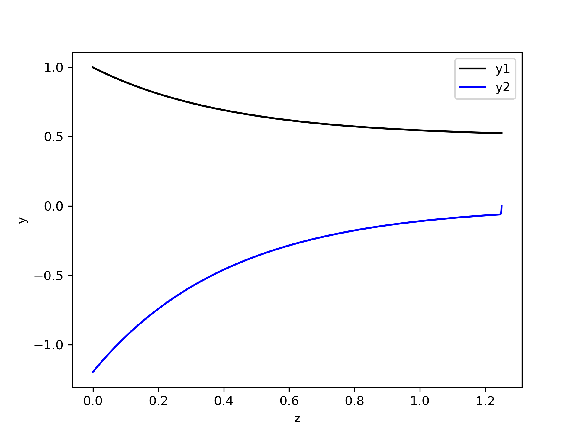
In this example, the BVODE solver did converge when the initial guess was that \(y_1\) and \(y_2\) equal zero at every mesh point. If it hadn’t, the engineer could have guessed the average values of \(y_1\) and \(y_2\) in the reactor, and used those values at all of the mesh points. (Of course, the engineer would know the physical significance of \(y_1\) and \(y_2\) when doing this.) It should also be noted that the initial mesh consisted of 20 mesh points, but the solver returned a mesh with more than 20 mesh points.
M.5 Symbols Used in Appendix M
| Symbol | Meaning |
|---|---|
| \(a\) | Lower limit of the independent variable or, undetermined coefficient in an approximating function, in which case a subscript indexes the approximating function. |
| \(b\) | Upper limit of the independent variable or, undetermined coefficient in an approximating function, in which case a subscript indexes the approximating function. |
| \(c\) | Undetermined coefficient in an approximating function, a subscript indexes the approximating function. |
| \(d\) | Undetermined coefficient in an approximating function, a subscript indexes the approximating function. |
| \(k\) | Known constant (rate coefficient) in Example M.4.1. |
| \(u_s\) | Known constant (superficial velocity) in Example M.4.1. |
| \(y\) | Dependent variable; a subscript denotes which variable when there are more than one; a second subscript denotes the mesh point. |
| \(z\) | Independent variable, a subscript denotes the value at a particular mesh point. |
| \(C_{A,0}\) | Known constant (inlet concentration of A) in Example M.4.1. |
| \(D\) | Known constant (dispersion coefficient) in Example M.4.1. |
| \(K\) | Known constant (equilibrium constant) in Example M.4.1. |
| \(L\) | Known constant (reactor length) in Example M.4.1. |
| \(N\) | Number or mesh points or subintervals. |
| \(\epsilon\) | Residual. |