25 Zoned Reactor Models
The last steady-state non-ideal reactor model type considered in Reaction Engineering Basics is the zoned reactor model, sometimes also called a compartment model. In effect, zoned reactor models are multiple reactor networks that are being used to model a single physical reactor. As such, the analysis of zoned reactors is essentially the same as the analysis of a reactor network as described in Chapter 15. Typically zoned reactor models include several unknown parameters that need to be estimated.
25.1 Using a Reactor Network to Model a Non-Ideal Reactor
Sometimes a reactor that is expected to obey the assumptions of an ideal reactor fails to do so. A reaction engineer may suspect that there is a physical issue that causes the flow to be different from that in an ideal reactor. In this situation, the engineer has two options. One is to try to correct the physical issue so that the reactor does obey the ideal reactor model. This will likely require shutting the reactor down while the issue is being addressed. Shutting the reactor down, in turn, will affect the company’s profits.
If the performance of the reactor is acceptable, but not equal to the predictions from an ideal reactor model, it may be beneficial, instead, to determine whether a zoned reactor model can accurately describe the non-ideal reactor. The zoned reactor model will include unknown parameters that need to be estimated. As discussed later, it may be possible to estimate the parameters without interrupting the operation of the reactor.
The zoned reactor model usually includes the inaccurate ideal reactor model, but adds a second reactor to it. The resulting two-reactor network is then used as a model for the single non-ideal reactor. The individual reactors in the network are called zones or compartments. There can be any number of zones, but generally the number of zones is small because each added zone introduces several unknown parameters that must be estimated.
There are no hard and fast rules regarding the zones. For example, the inaccurate ideal reactor model does not have to be used as a zone. As indicated in the discussion below, a zoned model is used, and the zones are selected, because the engineer suspects a physical issue that is causing the flow or mixing to deviate from ideal, and the zone or zones are added to try to account for that physical issue.
25.1.1 Reactor Zone Types
Each zone in a zoned reactor model is either an ideal CSTR or an ideal PFR. Individually they are modeled using the ideal reactor design equations (see Chapters 12 and 13). What varies from one zoned reactor model to the next are the specific ideal reactors and how they are connected. Three basic types of connection will cover a majority of situations.
The first two types connections between zones are parallel and series. These have already been considered in Chapter 15. The third type of connection creates a “well mixed stagnant” zone by use of a CSTR zone. The inlet to a well mixed stagnant zone and the outlet from it both connect to another reactor zone at the same location. In effect, the well mixed stagnant CSTR zone draws some amount of fluid out of the reactor zone it is connected to while simultaneously replacing that withdrawn fluid with an equal amount taken from the well-mixed stagnant CSTR zone.
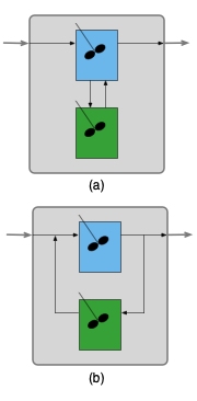
Figure 25.1 (a) shows a zoned reactor model where a well-mixed stagnant CSTR zone has been added to an ideal CSTR zone. Note the inlet to the stagnant zone is drawn from the regular CSTR’s contents and the outlet from the stagnant zone feeds back into the regular CSTR’s contents. Noting that the contents of the regular CSTR zone are perfectly mixed, the feed into the stagnant zone could equally well be drawn from the outlet of the regular CSTR zone and the outlet from the stagnant zone could equally well be added to the feed to the regular CSTR zone as shown in (b). The two representations are equivalent, but the latter is more convenient for writing design equations for the zoned reactor. With that schematic, the design equations consist of the CSTR design equations for the reactor, the CSTR design equations for the stagnant zone, mole and energy balances on the stream splitting point and mole and energy balances on the stream mixing point.
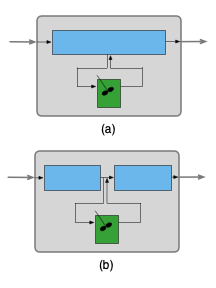
Similarly, Figure 25.2 (a) shows a zoned reactor model where a well-mixed stagnant CSTR zone has been added to an ideal PFR zone. To facilitate analysis (b), the single PFR zone can be split into two PFR zones connected in series. Here the design equations for the zoned reactor model include the PFR design equations for the reactor, the CSTR design equations for the stagnant zone, mole and energy balances on the stream splitting point and mole and energy balances on the stream mixing point.
Well-mixed stagnant zones have been emphasized here because they are not encountered anywhere else in this book. However, zoned reactor models are not required to include a well-mixed stagnant zone. As seen below, they may include two or more ideal flow reactors.
25.1.2 Selecting and Connecting Reactor Zones
Developing a zoned reactor model requires some insight into the reason why the reactor being modeled does not obey the ideal reactor assumptions. A few examples are considered in this section.
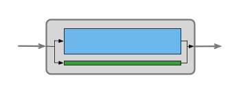
Suppose the catalyst in a packed bed reactor had to be replaced. Before the replacement the reactor performance was accurately described by the ideal PFR model, but after the change, the ideal PFR model is no longer sufficiently accurate. This might lead an engineer to suspect that the new catalyst packing is not properly distributed in the reactor and as a consequence, a fraction of the flow is bypassing part of the packed bed. This might be modeled as a two zone reactor consisting of two PFRs in parallel, as indicated schematically in Figure 25.3. Most of the flow in the model would pass through a PFR zone that represents the packed bed, while an appropriate fraction of the flow would pass through the other PFR zone that represents the bypassing flow.
Alternatively, the engineer might suspect that maldistribution of the packing has created a well-mixed stagnant zone within the packed bed. In that case Figure 25.2 might be used to model the non-ideal reactor.
A third possibility might be that measurement of the cumulative age distribution function indicates some mixing in the axial direction. One option then would be to model the reactor using an axial dispersion model (see Chapter 24). Alternatively, recalling (Chapter 15) that an infinite number of CSTRs connected in series is equivalent to a PFR, the non-ideal reactor might be to use a zoned reactor model where some number of equally-sized CSTR zones are connected in series. Depending on the number of CSTRs in series, this zoned reactor model can predict a range of behaviors from that of a single CSTR to that of an ideal PFR.
Zoned reactor models are not limited to non-ideal tubular reactors, they can be used to model non-ideal stirred tank reactors, too. For example, if the agitation in a stirred tank is not functioning properly there might be pockets” of fluid that are not perfectly mixed with the rest of the fluid in the reactor. This reactor might be modeled as a CSTR in combination with a well-mixed stagnant zone.
25.2 Zoned Reactor Model Parameters
Each time a reactor zone is added to a zoned reactor model, unknown parameters are added to the model. Consider Figure 25.1 as an example. Adding the well-mixed stagnant zone to the model introduces at least two parameters. One new parameter is the fraction of the fluid leaving the CSTR that is directed to the well-mixed stagnant CSTR zone. A second new parameter is the space time (or volume) of the well-mixed stagnant CSTR zone. If the non-ideal reactor exchanges heat with an external heating or cooling fluid, the relative heat transfer areas associated with the ideal CSTR and the stagnant zone CSTR becomes another parameter. Additionally, it isn’t required that the combined volumes or heat transfer areas of the zones must equal those of the non-ideal reactor. In the case that they do not equal the non-ideal reactor, two more unknown parameters are added.
When a zone is added to a model containing an ideal PFR zone, the same set of parameters is introduced along with one additional parameter. Referring to Figure 25.2, the additional parameter is the axial distance from the inlet of the ideal PFR zone where the well-mixed stagnant zone connects. Similarly, Figure 25.3 shows the feed splitting between the packed bed zone and the bypassing zone at the inlet and recombining at the outlet. In fact, the bypassing zone might start some distance into the packed bed zone and/or end some distance before the end of the packed bed zone.
The important points are that zoned reactor models typically contain several unknown parameters and each of those parameters must be estimated before the model can be used. This is a good reason for using the smallest possible number of zones, ideally just two. If the model contains too many parameters, it is difficult to estimate values for all of them, and the model can lose its predictive accuracy at conditions different from those used to estimate the parameters.
An engineer can reduce the number of estimated parameters by choosing fixed values for some of them. For example, an engineer could simply decide that the split into a packed bed zone and a bypass zone occurs at the reactor inlet and they merge at the reactor outlet in Figure 25.3. Similarly an engineer could simply decide that 10% of the fluid leaving a perfect CSTR is fed to a well-mixed stagnant zone or the engineer could set the volumes of the ideal CSTR and well-mixed stagnant zones.
Simply choosing some parameter values and estimating the rest is acceptable as long as the resulting zoned reactor model accurately describes the performance of the non-ideal reactor. Zoned reactor models are empirical. The parameter values have no theoretical basis, so as long as the model is accurate, it is acceptable.
That leaves the question of how to estimate the remaining parameters. If the non-ideal reactor can be shut down and then used for experiments, the zoned reactor model parameters could be estimated in the same way that rate expression parameters are estimated. A number of experiments could be performed, varying inputs to the reactor with a response being measured for each experiment. The non-ideal reactor model then could be used to create a predicted responses model (see Chapters 18 through 21) which could be fit to the data.
Very often, however, the reactor cannot be shut down and used for experiments. One option in that situation is to measure the cumulative age distribution function. A transient version of the zoned reactor model then could be fit to the age function data to estimate the parameters. This approach will not be illustrated in this chapter because Reaction Engineering Basics does not consider the analysis of transient reactor networks. The estimation of zoned reactor model parameters is left for an intermediate book on reaction engineering.
25.3 Examples
Two simple examples of zoned reactor models are presented in this section. The first is a zoned reactor model for a packed bed where bypassing is suspected. The other is a zoned reactor model for a stirred tank with a well-mixed stagnant zone.
25.3.1 A Zoned Reactor Model for Bypassing in a Packed Bed
A tube that is 6 m long with an inside diameter of 7 cm is packed with pellets of solid catalyst. Reaction (1) takes place within this reactor at a constant temperature of 450 ºC and a constant pressure of 5 atm. The tube will be fed 200 ft3 h-1 of a gas containing 15% A, 15% B and 70% I (an inert gas). Reaction (1) is one-half order in A and first order in B as indicated in equation (2). Suppose that the packing in the tube is not uniform, and as a consequence 5% of the bed has a lower density (leading to a rate coefficient of 1785 mol h-1 atm-0.5 m-3), while the remainder has a higher density (with a rate coefficient of 2160 mol h-1 atm-0.5 m-3). Using a zoned reactor model with two parallel PFR zones, show how the conversion will vary as the fraction of the feed gas flowing into the less dense part of the bed varies between 0 and 25%. Discuss the parameters in this zoned reactor model and how they might be estimated.
\[ 2A + B \rightarrow 2 Z \tag{1} \]
\[ r = k P_B \sqrt{P_A} \tag{2} \]
In this assignment I’m asked to examine the effect of varying a parameter in a zoned reactor model on the conversion predicted by the model. I’ll begin by summarizing the assignment. There are two zones in the model, I’ll designate the one with a higher packing density as “R1”, and the other as R2. I’ll use \(f_{f,R2}\) to designate the fraction of the feed that goes to the low density zone and $f_{V,R2} to designate the fraction of the bed volume corresponding to the low density zone. Finally, I’ll use an overbar to designate sets of values of a quantity.
25.3.1.1 Assignment Summary
Reaction:
\[ 2A + B \rightarrow 2 Z \tag{1} \]
Rate Expression:
\[ r = k P_B \sqrt{P_A} \tag{2} \]
Reactor System: Zoned Reactor with Two Ideal PFR Zones
Reactor Schematic:
Quantities of Interest: \(\overline{f}_A\) vs. \(\overline{f}_{f,R2}\)
Given and Known Constants: \(L_{NI}\) = 6 m, \(D_{NI}\) = 7 cm, \(T\) = 450 ºC, \(P\) = 5 atm, \(\dot{V}_0\) = 200 ft3 h-1, \(y_{A,0}\) = 0.15, \(y_{B,0}\) = 0.15, \(y_{I,0}\) = 0.70, \(f_{V,R2}\) = 0.05, \(k_{R2}\) = 1785 mol h-1 atm-0.5 m-3, \(k_{R1}\) = 2160 mol h-1 atm-0.5 m-3.
25.3.1.2 Mathematical Formulation of the Analysis
The formulation that follows assumes that the given and known constants identified in the assignment summary are available at any point in the analysis.
In the model, the reaction actually takes place in two ideal PFR zones. I’ll start by generating a PFR zone model that can be used to simulate either of the two zones. The zones are isothermal at a known temperature, so all I need to model them are mole balances. Since the feed to the zones and the volumes of the zones are different, these will be passed to the function at the time the zone is simulated.
The general form of the steady-state PFR mole balance is given in Equation 6.33. Here the PFR zones operate at steady-state, so all of the time derivatives equal zero, and the spatial derivative is an ordinary derivative. I don’t know the diameters of the separate zones, so I’ll re-write the mole balance in terms of the cumulative zone volume. Additionally, there is only one reaction, so the summation reduces to a single term and it isn’t necessary to index the reaction.
\[ \cancelto{\frac{d\dot{n}_i}{dz}}{\frac{\partial \dot{n}_i}{\partial z}} + \frac{\pi D^2}{4\dot{V}} \cancelto{0}{\frac{\partial\dot{n}_i}{\partial t}} - \frac{\pi D^2\dot{n}_i}{4\dot{V}^2} \cancelto{0}{\frac{\partial \dot{V}}{\partial t}} =\frac{\pi D^2}{4}\cancelto{\nu_t r}{\sum_j \nu_{i,j}r_j} \]
\[ \frac{d\dot{n}_i}{dz} = \frac{\pi D^2}{4}\nu_ir \qquad \Rightarrow \qquad \frac{d\dot{n}_i}{\frac{\pi D^2}{4}dz} = \nu_ir \qquad \Rightarrow \qquad \frac{d\dot{n}_i}{dV} = \nu_ir \]
The design equations will be solved numerically using an IVODE solver. I’ll need to provide initial values, a stopping criterion, and a derivatives function to the solver.
I can define \(V=0\) to be the inlet to the zone in which case the initial values simply equal the inlet molar flow rates to the zone. Since I’ll be using the same reactor model for both zones, these will be provided as arguments. Similarly, the stopping criterion then is that the final value of the volume is the volume of the zone. Again, this will need to be provided as an argument.
Design Equations
\[ \frac{d\dot{n}_A}{dV} = -2r \tag{3} \]
\[ \frac{d\dot{n}_B}{dV} = -r \tag{4} \]
\[ \frac{d\dot{n}_Z}{dV} = 2r \tag{5} \]
\[ \frac{d\dot{n}_I}{dV} = 0 \tag{6} \]
Initial Values and Stopping Criterion:
| Variable | Initial Value | Stopping Criterion |
|---|---|---|
| \(V\) | \(0\) | \(V_f\) |
| \(\dot{n}_A\) | \(\dot{n}_{A,in}\) | |
| \(\dot{n}_B\) | \(\dot{n}_{B,in}\) | |
| \(\dot{n}_Z\) | \(0.0\) | |
| \(\dot{n}_I\) | \(\dot{n}_{I,in}\) |
I also must write a derivatives function that I can provide to the IVODE solver. When the solver calls the derivatives function, the only arguments it will pass are the values of the independent and dependent and dependent variables at the start of an integration step, and the only return values it will expect to receive are the derivatives of the dependent variables with respect to the independent variable. Looking at the design equations, I see that I will need to calculate the rate. I can use the rate expression to do that. The partial pressures of A and B in the rate expression can be calculated as their mole fractions times the total pressure.
I will also need the rate coefficient, but the correct value will depend upon which reactor is being modeled. I can’t pass the correct rate coefficient to the derivatives function as an argument, so I’ll need to make sure to make it available by some other means.
Derivatives Function:
Arguments: \(V\), \(\dot{n}_A\), \(\dot{n}_B\), \(\dot{n}_Z\), \(\dot{n}_I\)
Must be Available: \(k\)
Returns: \(\frac{d\dot{n}_A}{dV}\), \(\frac{d\dot{n}_B}{dV}\), \(\frac{d\dot{n}_Z}{dV}\), \(\frac{d\dot{n}_I}{dV}\)
Algorithm:
\[ P_A = \frac{\dot{n}_A}{\dot{n}_A + \dot{n}_B + \dot{n}_Z + \dot{n}_I}P \tag{7} \]
\[ P_B = \frac{\dot{n}_B}{\dot{n}_A + \dot{n}_B + \dot{n}_Z + \dot{n}_I}P \tag{8} \]
\[ r = k P_B \sqrt{P_A} \tag{2} \]
\[ \frac{d\dot{n}_A}{dV} = -2r \tag{3} \]
\[ \frac{d\dot{n}_B}{dV} = -r \tag{4} \]
\[ \frac{d\dot{n}_Z}{dV} = 2r \tag{5} \]
\[ \frac{d\dot{n}_I}{dV} = 0 \tag{6} \]
Now I can generate a PFR zone function. It will receive the inlet molar flow rates of the reagents and the volume of whichever PFR zone is being modeled. I have a choice regarding the rate coefficient. I can either pass the correct rate coefficient to this function as an argument, and then make it available to the derivatives function within this function, or I can make it available to the derivatives function before I call this function. I prefer passing it to this function as an argument, so that’s how I’ll structure the PFR Zone Function.
Solving the PFR design equations will yield corresponding sets of values of \(V\), \(\dot{n}_A\), \(\dot{n}_B\), \(\dot{n}_Z\), and \(\dot{n}_I\), that span the range from \(V=0\) to \(V=V_f\). In keeping with the practice used when modeling PFR elsewhere in the book, I’ll have this function return those profiles.
PFR Zone Function:
Arguments: \(\dot{n}_{A,in}\), \(\dot{n}_{B,in}\), \(\dot{n}_{Z,in}\), \(\dot{n}_{I,in}\), \(V_f\), and \(k\).
Returns: \(\overline{V}\), \(\dot{n}_{A}\), \(\dot{n}_{B}\), \(\dot{n}_{Z}\), \(\dot{n}_{I}\)
Algorithm:
\[ k \, \Rightarrow \, \text{available to Derivatives Function} \tag{9} \]
\[ \begin{matrix} \text{Initial Values, Stopping Criterion, Derivatives Function} \\ \Downarrow \\ \text{IVODE Solver} \\ \Downarrow \\ \overline{V}, \overline{\dot{n}}_A, \overline{\dot{n}}_B, \overline{\dot{n}}_Z, \overline{\dot{n}}_I \end{matrix} \tag{10} \]
There are several ways I could structure the remaining calculations. I’m going to write a zoned reactor function that calculates the outlet molar flow rates of the reagents. I’ll pass the fraction of the feed flowing to the low density zone as an argument.
Knowing the feed to the non-ideal reactor, the feeds to the two zones can be calculated directly.
\[ \dot{n}_{i,1} = \left(1 - f_{f,R2}\right)\dot{n}_{i,0} \]
\[ \dot{n}_{i,2} = f_{f,R2}\dot{n}_{i,0} \]
Those values, along with the appropriate reactor volume and rate coefficient can then be passed to the PFR Zone Function to get the molar flow rate profiles for each of the zones. After extracting the outlet molar flow rates from the profiles, they can be combined to find the outlet molar flow rates from the zoned reactor.
Argument: \(f_{f,R2}\)
Returns: \(\dot{n}_{A,5}\), \(\dot{n}_{B,5}\), \(\dot{n}_{Z,5}\), \(\dot{n}_{I,5}\)
Algorithm:
\[ \dot{n}_{i,0} = y_{i,0}\frac{P\dot{V}_0}{RT} \,; i = A, B, Z, \text{ and } I \tag{11} \]
\[ \dot{n}_{i,1} = \left(1 - f_{f,R2}\right)\dot{n}_{i,0} \,; i = A, B, Z, \text{ and } I \tag{12} \]
\[ V_{NI} = \frac{\pi D_{NI}^2 L_{NI}}{4} \tag{13} \]
\[ V_f = \left(1 - f_{V,R2}\right) V_{NI} \tag{14} \]
\[ k = k_{R1} \tag{15} \]
\[ \begin{matrix} \dot{n}_{A,1}, \dot{n}_{B,1}, \dot{n}_{Z,1}, \dot{n}_{I,1}, V_f, k \\ \Downarrow \\ \text{PFR Zone Function} \\ \Downarrow \\ \overline{V}, \overline{\dot{n}}_A, \overline{\dot{n}}_B, \overline{\dot{n}}_Z, \overline{\dot{n}}_I \end{matrix} \tag{16} \]
\[ \dot{n}_{i,3} = \overline{\dot{n}}_i \bigg\vert_{V=V_f} \,; i = A, B, Z, \text{ and } I \tag{17} \]
\[ \dot{n}_{i,2} = f_{f,R2}\dot{n}_{i,0} \,; i = A, B, Z, \text{ and } I \tag{18} \]
\[ V_f = f_{V,R2} V_{NI} \tag{19} \]
\[ k = k_{R2} \tag{20} \]
\[ \begin{matrix} \dot{n}_{A,3}, \dot{n}_{B,3}, \dot{n}_{Z,3}, \dot{n}_{I,3}, V_f, k \\ \Downarrow \\ \text{PFR Zone Function} \\ \Downarrow \\ \overline{V}, \overline{\dot{n}}_A, \overline{\dot{n}}_B, \overline{\dot{n}}_Z, \overline{\dot{n}}_I \end{matrix} \tag{21} \]
\[ \dot{n}_{i,4} = \overline{\dot{n}}_i \bigg\vert_{V=V_f} \,; i = A, B, Z, \text{ and } I \tag{22} \]
\[ \dot{n}_{i,5} = \dot{n}_{i,3} + \dot{n}_{i,4} \,; i = A, B, Z, \text{ and } I \tag{23} \]
All that remains now is to choose a range of values for \(\f_{f,R2}\) between 0 and 25%, solve the zoned reactor model for each value, and use the resulting outlet molar flow rate of A to calculate the conversion.
Algorithm:
\[ \text{Choose } \overline{f}_{f,R2} \text{ with } 0 \le f_{f,R2,k} \le 0.25 \tag{24} \]
\[ \dot{n}_{i,0} = y_{i,0}\frac{P\dot{V}_0}{RT} \,; i = A, B, Z, \text{ and } I \tag{11} \]
Repeat (25) and (26) for each \(f_{f,R2,k}\) in \(\overline{f}_{f,R2}\).
\[ \begin{matrix} f_{f,R2,k} \\ \Downarrow \\ \text{Zoned Reactor Function} \\ \Downarrow \\ \dot{n}_{A,5}, \dot{n}_{B,5}, \dot{n}_{Z,5}, \dot{n}_{I,5} \end{matrix} \tag{25} \]
\[ f_{A,k} \text{ in } \overline{f}_A = \frac{\dot{n}_{A,0} - \dot{n}_{A,5}}{\dot{n}_{A,0}} \tag{26} \]
25.3.1.3 Results, Analysis and Discussion
The calculations were performed as described above. Specifically the derivatives function, PFR zone function, and zoned reactor functions were written using a mathematics software package. A vector containing 100 values of \(f_{f,R2}\) between 0 and 25% was created. Each value was passed to the zoned reactor function to get the corresponding molar flow rate of reagent A in stream 5, and the overall conversion of A was calculated using equation (26). The results are plotted in Figure 25.5.
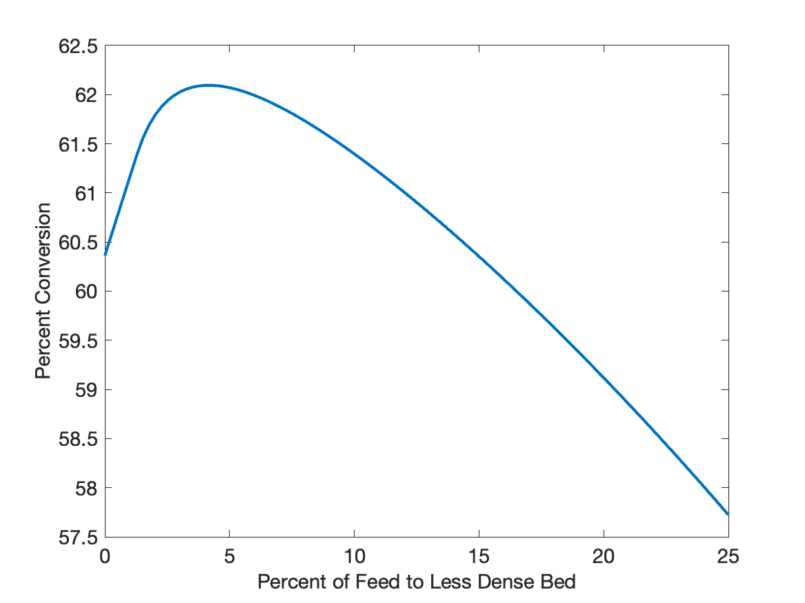
Intuitively one might expect the conversion to drop steadily as more and more of the flow bypasses the dense bed, but Figure 25.5 show that initially the conversion increases and then passes through a maximum before it starts to decrease steadily. Looking at the figure it can be seen that when all of the flow passes through the dense bed (\(\f_{f,R2}=0\)), the conversion is around 60.4%. When a small fraction of the feed flows to the less dense part of the bed, its space time in that bed will be very large because the flow is small. As a consequence, the part of the flow passing through the less dense bed may have a conversion approaching 100%.
At the same time, this decreases the space time of the fluid in the dense bed, causing its conversion to increase, too. Thus, when the two flows are combined, the conversion greater than it would have been had all of the flow passed through the dense bed. Eventually, as more an more of the flow passes into the less dense bed the conversions in the two beds becomes equal. This corresponds to the maximum in Figure 25.5. A further increase in \(\f_{f,R2}\) increases the space time such that the final conversion is less than that in the less dense bed, so when the streams are combined, the conversion decreases.
25.3.2 A Zoned Reactor Model for a CSTR with a Stagnant Zone
Reactants A and B can react irreversibly to produce either a desired product, D, or an undesired product, U, as shown in equations (1) and (2). The corresponding rate expressions are given in equations (3) and (4). The pre-exponential factors for \(k_1\) and \(k_2\) are 10.2 gal mol-1 min-1 and 17.0 gal mol-1 min-1, respectively, and the activation energies are 15.3 kJ mol-1 and 23.7 kJ mol-1, respectively. A liquid mixture containing 10 mol A gal-1 and 12 mol B gal-1 at 350 K is fed to an adiabatic 25 gal CSTR at a rate of 12.5 gal min-1. Example 12.7.1 showed that if the standard heats at 298 K of reactions (1) and (2) are -12.0 and -21.3 kJ mol-1, respectively, and if the reagents form an ideal liquid mixture with the temperature-independent heat capacities of A, B, D and U equal to 85, 125, 200 and 170 J mol-1 K-1, then the conversion of A is 54.9%, the selectivity is 8.39 mol D per mol U, and the outlet temperature is 383 K. How will these results change if 5% of the CSTR volume is a well-mixed stagnant zone that exchanges fluid with the remainder of the reactor at a rate of 0.5 gal min-1?
\[ A + B \rightarrow D \tag{1} \]
\[ A + B \rightarrow U \tag{2} \]
\[ r_1 = k_1 C_AC_B \tag{3} \]
\[ r_2 = k_2 C_AC_B \tag{4} \]
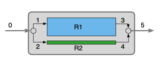
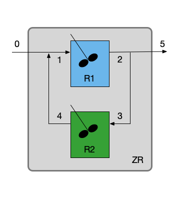
This assignment involves a CSTR with a well-mixed stagnant zone, so I’ll be using a zoned reactor model. I’ll begin by summarizing the assignment. For the schematic I’ll use Figure 25.1 (b) since it shows a vlow mixing point and a flow splitting point. I’ll use “ZR” to designate the non-ideal stirred tank that is being modeled using a zoned reactor model, “R1” to designate the CSTR zone, and “R2” to designate the well-mixed stagnant zone. The reactor operates at steady-state and the fluid is an incompressible liquid, so the fluid exchange rate given in the narrative is equal to the flow into and out of the stagnant zone.
25.3.2.1 Assignment Summary
Reactions:
\[ A + B \rightarrow D \tag{1} \]
\[ A + B \rightarrow U \tag{2} \]
Rate Expressions:
\[ r_1 = k_1 C_AC_B \tag{3} \]
\[ r_2 = k_2 C_AC_B \tag{4} \]
Reactor System: Zoned reactor with a CSTR zone and a well-mixed stagnant zone.
Reactor Schematic:
Quantities of Interest: \(f_A\), \(S_{D/U}\), and \(T_5\)
Given and Known Constants: \(k_{0,1}\) = 10.2 gal mol-1 min-1, \(k_{0,2}\) = 17.0 gal mol-1 min-1, \(E_1\) = 15.3 kJ mol-1, \(E_2\) = 23.7 kJ mol-1, \(C_{A,0}\) 10 mol A gal-1, \(C_{B,0}\) = 12 mol B gal-1, \(T_0\) = 350 K, \(V_{ZR}\) = 25 gal, \(\dot{V}_0\) = 12.5 gal min-1, \(\Delta H_1\) = -12.0, \(\Delta H_2\) = -21.3 kJ mol-1, \(\hat{C}_{p,A}\) = 85, \(\hat{C}_{p,B}\) = 125, \(\hat{C}_{p,D}\) = 200, \(\hat{C}_{p,U}\) = 170 J mol-1 K-1, \(f_{R2}\) = 0.05, and \(\dot{V}_{3}\) = \(\dot{V}_{4}\) = 0.5 gal min-1.
25.3.2.2 Mathematical Formulation of the Analysis
The formulation that follows assumes that the given and known constants identified in the assignment summary are available at any point in the analysis.
The reaction actually takes place within the CSTR zone and the well-mixed stagnant zone. Both of those zones are modeled using the ideal CSTR design equations. Before I can write design equations, I need to make an assumption about heat transfer between the two zones. Overall the stirred tank is adiabatic, but the two zones must be in contact within the reactor. To avoid having to guess both the contact area and the heat transfer coefficient between the two zones, I’m simply going to assume them both to be adiabatic.
Since both zones are being modeled as ideal CSTRs, I’m going to use the same CSTR zone model for each of them. That means that the volume, inlet volumetric flow rate, inlet temperature, and inlet composition will need to be provided to the model. Since I’ve assumed the two zones to each be adiabatic, I’ll need mole balances on each of the reagents and an energy balance on the reacting fluid as reactor design equations.
The general form of a steady-state CSTR mole balance is given in Equation 6.31. Two reactions taking place, so the summation expands to two terms.
\[ 0 = \dot{n}_{i,in} - \dot{n}_{i,out} + V \sum_j \nu_{i,j}r_j = \dot{n}_{i,in} - \dot{n}_{i,out} + V \left( \nu_{i,1}r_1 + \nu_{i,2}r_2 \right) \]
The general form of a steady-state CSTR energy balance is given in Equation 6.32. Assuming the zone to be adiabatic means the heat exchange term is equal to zero, and assuming the power required to agitate the fluid to be neglible means the work term is zero. The heat capacities are constants, so they can be factored out of the integrals and the integrals can be evaluated analytically. Finally, as above, there are two reactions, so the final sum expands to two terms.
\[ 0 = \cancelto{0}{\dot{Q}} - \cancelto{0}{\dot{W}} - \sum_i\dot{n}_{i,in} \cancelto{\hat{C}_{p,i}\left(T-T_{in}\right)}{\int_{T_{in}}^T \hat{C}_{p,i}dT} - V\cancelto{r_1 \Delta H_1 + r_2 \Delta H_2}{\sum_j r_j \Delta H_j} \]
\[ 0 = -\left(\begin{matrix}\dot{n}_{A,in} \hat{C}_{p,A} + \dot{n}_{B,in} \hat{C}_{p,B} \\ \dot{n}_{D,in} \hat{C}_{p,D} + \dot{n}_{U,in} \hat{C}_{p,U} \end{matrix}\right) \left(T-T_{in}\right) - V\left(r_1 \Delta H_1 + r_2 \Delta H_2\right) \]
The mole and energy balance design equations are ATEs, and they will be solved numerically using an ATE solver to find the outlet molar flow rates and the outlet temperature. To do that, I’ll need to provide a guess for the solution and a residuals function to the solver. In anticipation of writing the residuals function, the design equations are written as residual expressions.
Design Equations
\[ 0 = \epsilon_A = \dot{n}_{A,in} - \dot{n}_{A,out} + V \left( -r_1 -r_2 \right) \tag{5} \]
\[ 0 = \epsilon_B = \dot{n}_{B,in} - \dot{n}_{B,out} + V \left( -r_1 -r_2 \right) \tag{6} \]
\[ 0 = \epsilon_D = \dot{n}_{D,in} - \dot{n}_{D,out} + V r_1 \tag{7} \]
\[ 0 = \epsilon_U = \dot{n}_{U,in} - \dot{n}_{U,out} + V r_2 \tag{8} \]
\[ 0 = \epsilon_T = \left(\begin{matrix}\dot{n}_{A,in} \hat{C}_{p,A} + \dot{n}_{B,in} \hat{C}_{p,B} \\ \dot{n}_{D,in} \hat{C}_{p,D} + \dot{n}_{U,in} \hat{C}_{p,U} \end{matrix}\right) \left(T-T_{in}\right) + V\left(r_1 \Delta H_1 + r_2 \Delta H_2\right) \tag{9} \]
I need to guess the outlet molar flow rates and the outlet temperature and provide the guess to the ATE solver. I’ll simply guess that A and B decrease by 10% producing equal amounts of D and U. The reaction is exothermic, so I’ll guess that the temperature increases by 10 K. If the solver doesn’t converge, I may need to adjust these guesses, or I may need to provide different guesses, depending upon which zone is being modeled.
Initial Guesses for \(\dot{n}_{A,out}\), \(\dot{n}_{B,out}\), \(\dot{n}_{D,out}\), \(\dot{n}_{U,out}\), and \(T_{out}\):
\[ \dot{n}_{A,out,guess} = 0.9\dot{n}_{A,in} \tag{10} \]
\[ \dot{n}_{B,out,guess} = 0.9\dot{n}_{B,in} \tag{11} \]
\[ \dot{n}_{D,out,guess} = 0.05\dot{n}_{A,in} \tag{12} \]
\[ \dot{n}_{U,out,guess} = 0.05\dot{n}_{A,in} \tag{13} \]
\[ T_{out,guess} = T_{in} + 10 \text{ K } \tag{14} \]
The other thing I need to provide to the ATE solver is a residuals function. The solver will call the residuals function passing guesses for the unknowns (and nothing else) as arguments, and it will expect the residuals function to return the corresponding values of the residuals (and nothing else).
Before the values of the residuals can be calculated, any other unknowns appearing in the design equations must first be calculated. Looking at the design equations, I see that \(\dot{n}_{A,in}\), \(\dot{n}_{B,in}\), \(\dot{n}_{D,in}\), \(\dot{n}_{U,in}\), \(V\), \(r_1\), and \(r_2\) are all unknown.
I can’t write equations to calculate the inlet molar flow rates and the reactor volume because when the residuals function is called, it could be evaluating the residuals for either the CSTR zone or the well-mixed stagnant zone. I can’t pass \(\dot{n}_{A,in}\), \(\dot{n}_{B,in}\), \(\dot{n}_{D,in}\), \(\dot{n}_{U,in}\), and \(V\) as arguments, so I’ll need to make them available in some other way.
I can use the rate expressions to calculate the rate expressions, but first I’ll need to calculate the concentrations of A and B. That can be done using the definition of concentration in an open system, Equation 2.15. To use that equation, however, I need the volumetric flow rate. I can’t calculate the volumetric flow rate because, again, it depends whether the the CSTR zone or the well-mixed stagnant zone is being analyzed. Therefore, \(\dot{V}\) will also need to be provided by some other means. The rate coefficients can be calculated using the Arrhenius expression, Equation 4.8.
CSTR Residuals Function:
Arguments: \(\dot{n}_{A,out}\), \(\dot{n}_{B,out}\), \(\dot{n}_{D,out}\), \(\dot{n}_{U,out}\), and \(T_{out}\)
Must be Available: \(\dot{n}_{A,in}\), \(\dot{n}_{B,in}\), \(\dot{n}_{D,in}\), \(\dot{n}_{U,in}\), \(V\), and \(\dot{V}\)
Returns: \(\epsilon_A\), \(\epsilon_B\), \(\epsilon_D\), \(\epsilon_U\), and \(\epsilon_T\)
Algorithm:
\[ C_A = \frac{\dot{n}_{A,out}}{\dot{V}} \tag{15} \]
\[ C_B = \frac{\dot{n}_{B,out}}{\dot{V}} \tag{16} \]
\[ k_1 = k_{0,1}\exp{\left(\frac{-E_1}{RT_{out}}\right)} \tag{17} \]
\[ k_2 = k_{0,2}\exp{\left(\frac{-E_2}{RT_{out}}\right)} \tag{18} \]
\[ r_1 = k_1 C_AC_B \tag{3} \]
\[ r_2 = k_2 C_AC_B \tag{4} \]
\[ 0 = \epsilon_A = \dot{n}_{A,in} - \dot{n}_{A,out} + V \left( -r_1 -r_2 \right) \tag{5} \]
\[ 0 = \epsilon_B = \dot{n}_{B,in} - \dot{n}_{B,out} + V \left( -r_1 -r_2 \right) \tag{6} \]
\[ 0 = \epsilon_D = \dot{n}_{D,in} - \dot{n}_{D,out} + V r_1 \tag{7} \]
\[ 0 = \epsilon_U = \dot{n}_{U,in} - \dot{n}_{U,out} + V r_2 \tag{8} \]
\[ 0 = \epsilon_T = \left(\begin{matrix}\dot{n}_{A,in} \hat{C}_{p,A} + \dot{n}_{B,in} \hat{C}_{p,B} \\ \dot{n}_{D,in} \hat{C}_{p,D} + \dot{n}_{U,in} \hat{C}_{p,U} \end{matrix}\right) \left(T-T_{in}\right) - V\left(r_1 \Delta H_1 + r_2 \Delta H_2\right) \tag{9} \]
Now that I have a guess for the solution and a residuals function, I can write the CSTR zone function to solve the design equations. I have two options regarding making \(\dot{n}_{A,in}\), \(\dot{n}_{B,in}\), \(\dot{n}_{D,in}\), \(\dot{n}_{U,in}\), \(V\), and \(\dot{V}\) available to the residuals function. I can either make them available before I call the CSTR zone function or I can pass them to the CSTR zone function as arguments, and then make them available before I call the solver. I prefer the latter, so that’s how I’ll proceede.
CSTR Zone Function:
Arguments: \(\dot{n}_{A,in}\), \(\dot{n}_{B,in}\), \(\dot{n}_{D,in}\), \(\dot{n}_{U,in}\), \(V\), and \(\dot{V}\)
Returns: \(\dot{n}_{A,out}\), \(\dot{n}_{B,out}\), \(\dot{n}_{D,out}\), \(\dot{n}_{U,out}\), and \(T_{out}\)
Algorithm:
\[ \dot{n}_{A,in}, \dot{n}_{B,in}, \dot{n}_{D,in}, \dot{n}_{U,in}, V, \text{ and } \dot{V} \, \Rightarrow \, \text{available to Residuals Function} \tag{19} \]
\[ \begin{matrix} \begin{matrix} \dot{n}_{A,out,guess}, \dot{n}_{B,out,guess}, \dot{n}_{D,out,guess}, \\ \dot{n}_{U,out,guess}, T_{out,guess},\text{ Residuals Function} \end{matrix} \\ \Downarrow \\ \text{ATE Solver} \\ \Downarrow \\ \dot{n}_{A,out}, \dot{n}_{B,out}, \dot{n}_{D,out}, \dot{n}_{U,out}, \text{ and } T_{out} \end{matrix} \tag{20} \]
The zoned reactor for this assignment includes a stream merge, an ideal CSTR zone, a stream split, and a well-mixed stagnant zone. Looking at Figure 25.6, it appears that the mole and energy balances for the stream split, CSTR zone, stream merge, and well-mixed stagnant zone are coupled. That is, I can’t solve the mole and energy balances for any one of them independently of the others.
Upon closer inspection, however, I can see that if I knew the composition and temperature of stream 4, I could solve the mole and energy balances for the stream merge for the composition and temperature of stream 1. Then I could solve the design equations for the CSTR zone to get the composition and temperature of stream 2. Then, knowing the fraction of the total flow that exchanges with the stagnant zone, I could calculate the compositions and temperatures of streams 3 and 5. Finally, knowing the composition and temperature of stream 3, I could solve the well-mixed stagnant zone design equations for the composition and temperature of stream 4.
This situation is analogous to a set of CVODEs except that all of the equations are ATEs. As such, I can solve the equations in a manner analogous to the solution of a set of CVODEs. Briefly, I’ll write the mole and energy balances for the stream merge, and I’ll solve them numerically for the molar flow rates and temperature of stream 1. The molar flow rates and temperature of stream 4 will also appear in the equations and will be unknown. However when I write a residuals function for solving the stream merge equations, it will be given a guess for stream 1. I can use that guess to solve the CSTR design equations, use that result together with the known fraction of the total flow that exchanges with the stagnant zone to calculate the composition and temperature of stream 3, use that to solve the well-mixed stagnant zone design equations for the composition and temperature of stream 4, and use that to evaluate the residuals. That all may sound confusing at first, but again, it is analogous to solving a set of CVODEs.
So I’ll start by generating a model for the stream merge. The mole balances for the stream merge simply require the outlet molar flow rate to equal the sum of the two inlet molar flow rates. Assuming that these equations will be solved numerically, I’ll write them as residual expressions.
\[ \dot{n}_{i,0} + \dot{n}_{i,4} = \dot{n}_{i,1} \qquad \Rightarrow \qquad 0 = \dot{n}_{i,0} + \dot{n}_{i,4} - \dot{n}_{i,1} \]
Assuming the stream merge to be adiabatic (and that all of the streams are liquids), the energy balance simply requires that the sum of the heat changes of the two inlet streams must equal zero. That is, the energy lost by one stream equals the energy gained by the other.
\[ 0 = \sum_i \dot{n}_{i,0} \int_{T_0}^{T_1} \hat{C}_{p,i}dT + \sum_i \dot{n}_{i,4} \int_{T_4}^{T_1} \hat{C}_{p,i}dT \]
Here the heat capacities are constant, so they can be factored out of the integrals and the integrals can be evaluated analytically.
\[ 0 = \sum_i \dot{n}_{i,0}\hat{C}_{p,i} \left(T_1 - T_0\right) + \sum_i \dot{n}_{i,4}\hat{C}_{p,i} \left(T_1 - T_4\right) \]
Design Equations
\[ 0 = \epsilon_{21} = \dot{n}_{A,0} + \dot{n}_{A,4} - \dot{n}_{A,1} \tag{21} \]
\[ 0 = \epsilon_{22} = \dot{n}_{B,0} + \dot{n}_{B,4} - \dot{n}_{B,1} \tag{22} \]
\[ 0 = \epsilon_{23} = \dot{n}_{D,4} - \dot{n}_{D,1} \tag{23} \]
\[ 0 = \epsilon_{24} = \dot{n}_{U,4} - \dot{n}_{U,1} \tag{24} \]
\[ 0 = \epsilon_{25} = \left(\begin{matrix} \dot{n}_{A,0}\hat{C}_{p,A} +\\ \dot{n}_{B,0}\hat{C}_{p,B} +\\ \dot{n}_{D,0}\hat{C}_{p,D} +\\ \dot{n}_{U,0}\hat{C}_{p,U} \end{matrix} \right) \left(T_1 - T_0\right) + \left( \begin{matrix} \dot{n}_{A,4}\hat{C}_{p,A} +\\ \dot{n}_{B,4}\hat{C}_{p,B} +\\ \dot{n}_{D,4}\hat{C}_{p,D} +\\ \dot{n}_{U,4}\hat{C}_{p,U} \end{matrix} \right) \left(T_1 - T_4\right) \tag{25} \]
There are five stream merge design equations (21) through (25), and they contain ten unknown quantities (molar flow rates of all species in stream 1 and 4, and temperatures of streams 1 and 4). The critical aspect of solving them is to choose \(\dot{n}_{A,1}\), \(\dot{n}_{B,1}\), \(\dot{n}_{D,1}\), \(\dot{n}_{U,1}\), and \(T_1\) as the unknowns to be found by solving these design equations.
The stream merge design equations will be solved numerically using an ATE solver. I’ll need to provide a guess for each of the unknowns and a residuals function to the ATE solver. For no particular reason, I’m going to guess that the molar flow rates in stream are each equal to the molar flow rate in stream 0 plus some small amount. For the temperature, I’ll guess it is 5 K greater than stream 0. These are just guesses; if the solver fails to converge, I’ll change them.
Initial Guesses for \(\dot{n}_{A,1}\), \(\dot{n}_{B,1}\), \(\dot{n}_{D,1}\), \(\dot{n}_{U,1}\), and \(T_1\):
\[ \dot{n}_{A,1,guess} = \dot{V}_0 C_{A,0} + 0.05\dot{V}_0 C_{A,0} \tag{26} \]
\[ \dot{n}_{B,1,guess} = \dot{V}_0 C_{B,0} + 0.05\dot{V}_0 C_{A,0} \tag{27} \]
\[ \dot{n}_{D,1,guess} = 0.05\dot{V}_0 C_{A,0} \tag{28} \]
\[ \dot{n}_{U,1,guess} = 0.05\dot{V}_0 C_{A,0} \tag{29} \]
\[ T_{1,guess} = T_0 + 5 \text{ K} \tag{30} \]
The other thing I need to do is to write a residuals function for solving the stream merge design equations using an ATE solver. When the ATE solver calls the residuals function it will pass values for the unknowns, \(\dot{n}_{A,1}\), \(\dot{n}_{B,1}\), \(\dot{n}_{D,1}\), \(\dot{n}_{U,1}\), and \(T_1\), and nothing else, and it will expect the return values to be the residuals, \(\epsilon_{21}\), \(\epsilon_{22}\), \(\epsilon_{23}\), \(\epsilon_{24}\), and \(\epsilon_{25}\), and nothing else.
Before I can evaluate and return the residuals, I must calculate any other unknowns that appear in the stream merge design equations. As already noted, \(\dot{n}_{A,4}\), \(\dot{n}_{B,4}\), \(\dot{n}_{D,4}\), \(\dot{n}_{U,4}\), and \(T_4\) are unknown and they appear in the design equations. Therefore I need to calculate their values.
To do so, I’ll first call the CSTR zone function to get the molar flow rates and temperature for stream 2. Since the reacting fluid is an incompressible liquid, the volumetric flow rates of streams 1 and 2 must be equal, and the volumetric flow rate of stream 1 must equal the combined volumetric flow rates of streams 0 and 4.
\[ V_2 = V_1 = V_0 + V_4 \]
The fraction of stream 2 that splits off as stream 3 can be calculated from the volumetric flow rates. Since it is only a stream split that equals the fraction of the molar flow rates in stream 2 that are split off into stream 3, and the temperature of streams 2 and 3 are equal.
\[ f_{exch} = \frac{V_3}{V_2} \]
\[ \dot{n}_{i,3} = f_{exch}\dot{n}_{i,2} \]
\[ T_3 = T_2 \]
Having calculated the molar flow rates and temperature of stream 3, the design equations for the well-mixed stagnant zone can be solved by calling the CSTR zone function. This will yield the molar flow rates and temperature for stream 4.
Finally, then, the stream merge residuals can be evaluated and their values returned.
Stream Merge Residuals Function:
Arguments: \(\dot{n}_{A,1}\), \(\dot{n}_{B,1}\), \(\dot{n}_{D,1}\), \(\dot{n}_{U,1}\), and \(T_1\)
Returns: \(\epsilon_{21}\), \(\epsilon_{22}\), \(\epsilon_{23}\), \(\epsilon_{24}\), and \(\epsilon_{25}\)
Algorithm:
\[ V_{R1} = \left(1-f_{R2}\right)V_{ZR} \tag{32} \]
\[ \dot{V}_1 = \dot{V}_0 + \dot{V}_4 \tag{33} \]
\[ \dot{V}_2 = \dot{V}_1 \tag{34} \]
\[ \begin{matrix} \dot{n}_{A,1}, \dot{n}_{B,1}, \dot{n}_{D,1}, \dot{n}_{U,1}, T_1, V_{R1}, \dot{V}_1 \\ \Downarrow \\ \text{CSTR Zone Function} \\ \Downarrow \\ \dot{n}_{A,2}, \dot{n}_{B,2}, \dot{n}_{D,2}, \dot{n}_{U,2}, T_2 \end{matrix} \tag{35} \]
\[ f_{exch} = \frac{\dot{V}_3}{\dot{V}_2} \tag{36} \]
\[ \dot{n}_{i,3} = f_{exch}\dot{n}_{i,2} \,; \, i = A, B, D, \text{ and } U \tag{37} \]
\[ T_3 = T_2 \tag{38} \]
\[ V_{R2} = f_{R2}V_{ZR} \tag{39} \]
\[ \begin{matrix} \dot{n}_{A,3}, \dot{n}_{B,3}, \dot{n}_{D,3}, \dot{n}_{U,3}, T_3, V_{R2}, \dot{V}_3 \\ \Downarrow \\ \text{CSTR Zone Function} \\ \Downarrow \\ \dot{n}_{A,4}, \dot{n}_{B,4}, \dot{n}_{D,4}, \dot{n}_{U,4}, T_4 \end{matrix} \tag{40} \]
\[ \dot{n}_{A,0} = C_{A,0}\dot{V}_0 \tag{41} \]
\[ \dot{n}_{B,0} = C_{B,0}\dot{V}_0 \tag{42} \]
\[ 0 = \epsilon_{21} = \dot{n}_{A,0} + \dot{n}_{A,4} - \dot{n}_{A,1} \tag{21} \]
\[ 0 = \epsilon_{22} = \dot{n}_{B,0} + \dot{n}_{B,4} - \dot{n}_{B,1} \tag{22} \]
\[ 0 = \epsilon_{23} = \dot{n}_{D,4} - \dot{n}_{D,1} \tag{23} \]
\[ 0 = \epsilon_{24} = \dot{n}_{U,4} - \dot{n}_{U,1} \tag{24} \]
Stream Merge Function:
Arguments: none
Returns: \(\dot{n}_{A,1}\), \(\dot{n}_{B,1}\), \(\dot{n}_{D,1}\), \(\dot{n}_{U,1}\), and \(T_1\)
Algorithm:
\[ \begin{matrix} \begin{matrix} \dot{n}_{A,1,guess}, \dot{n}_{B,1,guess}, \dot{n}_{D,1,guess}, \dot{n}_{U,1,guess}, \\ T_{1,guess}, \text{ and Stream Merge Residuals Function} \end{matrix} \\ \Downarrow \\ \text{ATE Solver} \\ \Downarrow \\ \dot{n}_{A,1}, \dot{n}_{B,1}, \dot{n}_{D,1}, \dot{n}_{U,1}, \text{and } T_1 \end{matrix} \]
At this point I can write a zoned reactor function to calculate the molar flow rates and temperature of stream 5. The first thing it needs to do is to call the stream merge function to get the molar flow rates and temperature of stream 1. Then it can call the CSTR zone function to get the molar flow rates and temperature of stream 2. Finally it can use the exchange fraction, defined earlier, to calculate the molar flow rates and temperature of stream 5.
The temperature of stream 5 is one of the quantities of interest. The conversion of A can be calculated using its definition, Equation 3.5, and the selectivity for D over U can be calculated from the stream 5 molar flow rates.
Arguments: none
Returns: \(\dot{n}_{A,5}\), \(\dot{n}_{B,5}\), \(\dot{n}_{D,5}\), \(\dot{n}_{U,5}\), and \(T_5\)
Algorithm:
\[ \begin{matrix} \text{Stream Merge Function} \\ \Downarrow \\ \dot{n}_{A,1}, \dot{n}_{B,1}, \dot{n}_{D,1}, \dot{n}_{U,1}, \text{and } T_1 \end{matrix} \]
\[ V_{R1} = \left(1-f_{R2}\right)V_{ZR} \tag{32} \]
\[ \dot{V}_1 = \dot{V}_0 + \dot{V}_4 \tag{33} \]
\[ \dot{V}_2 = \dot{V}_1 \tag{34} \]
\[ \begin{matrix} \dot{n}_{A,1}, \dot{n}_{B,1}, \dot{n}_{D,1}, \dot{n}_{U,1}, T_1, V_{R1}, \dot{V}_1 \\ \Downarrow \\ \text{CSTR Zone Function} \\ \Downarrow \\ \dot{n}_{A,2}, \dot{n}_{B,2}, \dot{n}_{D,2}, \dot{n}_{U,2}, T_2 \end{matrix} \tag{35} \]
\[ f_{exch} = \frac{\dot{V}_3}{\dot{V}_2} \tag{36} \]
\[ \dot{n}_{i,5} = \left(1-f_{exch}\right)\dot{n}_{i,2} \,; \, i = A, B, D, \text{ and } U \tag{43} \]
\[ T_5 = T_2 \tag{44} \]
Algorithm:
\[ \begin{matrix} \text{Zoned Reactor Function} \\ \Downarrow \\ \dot{n}_{A,5}, \dot{n}_{B,5}, \dot{n}_{D,5}, \dot{n}_{U,5}, \text{and } T_5 \end{matrix} \tag{45} \]
\[ f_A = \frac{\dot{V}_0C_{A,0} - \dot{n}_{A,5}}{\dot{V}_0C_{A,0}} \tag{46} \]
\[ S_{D/U} = \frac{\dot{n}_{D,5}}{\dot{n}_{U,5}} \tag{47} \]
25.3.2.3 Results, Analysis and Discussion
The calculations were performed as described above. Specifically the CSTR REsiduals Function, CSTR Zone Function, Stream Merge Residuals Function, Stream Merge Function, and Zoned Reactor Function were written using a mathematics software package. The Zoned Reactor Function was called to get the molar flow rates and temperature for stream 5, and the conversion and selectivity were calculated using equations (46) and (47). The results for the stirred tank with a well-mixed stagnant zone are compared to the results for an ideal PFR in Table 25.2.
| Ideal CSTR | Stirred Tank with Stagnant Zone | |
|---|---|---|
| Conversion (%) | 54.9 | 54.4 |
| Selectivity (D/U) | 8.39 | 8.35 |
| Temperature (K) | 383 | 383 |
Adding a well-mixed stagnant zone had negligible effect upon the reactor’s performance. If an engineer was modeling a real reactor where there was a significant difference and if the engineer felt that the difference was due to a stagnant zone, the engineer adjust the zoned reactor model. Both the relative volume of the stagnant zone, \(f_{R2}\), and the fluid exchange flows, \(\dot{V}_3 = \dot{V}_4\), could be varied to find a combination of values that approaches the actual reactor performance as closely as possible.
When the zoned reactor model was formulated, a choice had to be made regarding heat exchange between the two fluid zones. In an actual reactor with a stagnant zone, one would expect some degree of heat exchange because the zones are in physical contact. However adding heat exchange to the model requires the heat transfer area and the heat transfer coefficient. A small stagnant zone is expected to have a small effect upon reactor performance, and on that basis the decision to model the reactors as adiabatic zones can be justified.
25.4 Symbols Used in Chapter 25
| Symbol | Meaning |
|---|---|
| \(f_i\) | Fractional conversion of reagent \(i\). |
| \(f_{exch}\) | Fraction of the fluid flow directed to and returning from the stagnant zone. |
| \(f_{V,R2}\) | Fraction of the non-ideal reactor volume corresponding to zone R2. |
| \(f_{f,R2}\) | Fraction of the fluid flow directed to zone R2. |
| \(k\) | Rate coefficient. |
| \(k_0\) | Arrhenius pre-exponential factor. |
| \(\dot{n}\) | Molar flow rate; additional subscripts denote the reagent and the fluid stream. |
| \(r\) | Reaction rate; a subscript is used to index individual reactions when more than one occur. |
| \(y\) | Mole fraction; additional subscripts denote the reagent and the flow stream. |
| \(C\) | Concentration; additional subscripts denote the reagent and the flow stream. |
| \(\hat{C}_{p,i}\) | Molar heat capacity of reagent \(i\). |
| \(D\) | Diameter; a subscript identifies the vessel. |
| \(E\) | Arrhenius activation energy; a subscript is used to index individual reactions when more than one occur. |
| \(L\) | Length; a subscript identifies the vessel. |
| \(P\) | Pressure; a subscripted \(i\) indicates the partial pressure of reagent \(k\). |
| \(S_{D/U}\) | Selectivity for D over U. |
| \(T\) | Temperature; a subsript denotes the fluid stream. |
| \(V\) | Volume; an additional subscript denotes the reactor or zone. |
| \(\dot{V}\) | Volumetric flow rate; a subscript denotes the fluid stream. |
| \(\epsilon\) | Residual; a subscript is used to index the residuals when there are more than one. |
| \(\Delta H\) | Heat of reaction; a subscript is used to index individual reactions when more than one occur. |