17 Recycle PFRs
One of the most important factors when comparing different reactor systems is the way that the composition and temperature vary over the time during which the reaction is taking place. CSTRs and PFRs represent the two extremes. The temperature and composition are constant for the entire time the reaction is taking place in a CSTR, while they vary continuously over the time the reaction is taking place in a PFR.
Chapter 16 showed how, for an exothermic reaction, the variation of the temperature during the time the reaction is taking place in a PFR can be altered to be a little bit more like a CSTR. That is accomplished by transferring heat from the product stream to the feed stream. This chapter examines a way to alter the variation of both the temperature and the composition during the time the reaction is taking place in a PFR to be a little bit more like a CSTR. To accomplish that, a fraction of the product stream is split off and mixed with the process feed stream. A reactor with this configuration is called a recycle PFR.
17.1 Recycle PFRs
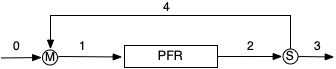
A recycle PFR is depicted in Figure 17.1. The system consists of a stream mixer, the PFR, and a stream splitter. The fluid stream, 2, leaving the reactor is split into two streams. One of the resulting streams, 3, is the product stream for the process. The other stream, 4, is called the recycle stream because it is diverted back to the reactor inlet where it is mixed with the fresh feed to the process, stream 0. The resulting mixed stream, 1, is what enters the PFR.
In a steady-state CSTR, the fresh feed is immediately mixed into the reacting fluid. As a consequence, the composition and temperature are at their outlet values for the entire time the fluid reacts. In a PFR, the composition and temperature change continuously as the fluid flows through the reactor starting at their inlet values and ending at their outlet values . By recycling, or backmixing, some of the converted fluid into the fresh feed, the inlet composition and temperature are effectively those of a partially converted feed stream.
Another way to describe the differences is that in a PFR the composition and temperature of the reacting fluid progress from their inlet values to their outlet values, while in a CSTR, the composition and temperature of the reacting fluid immediately jump to their outlet values. In a recycle PFR, then, the composition and temperature of the reacting fluid immediately jump part of the way to their outlet values and then progress the rest of the way to their outlet values. In that way, adding recycle to a PFR shifts it’s behavior to be more like a CSTR.
The ratio of the flow rate of stream 4 to that of stream 3 is called the recycle ratio, \(R_R\), Equation 17.1. As the recycle ratio approaches infinity, that is as more and more of stream 2 is recycled, a recycle PFR approaches the behavior of a CSTR. The recycle ratio can be calculated using volumetric flow rates or the molar flow rate of any reagent, \(i\), present in the system, as shown in the equation.
\[ R_R = \frac{\dot{V}_4}{\dot{V}_3} = \frac{\dot{n}_{i,4}}{\dot{n}_{i,3}} \tag{17.1}\]
Adding thermal backmixing to a PFR shifts it’s thermal behavior to be more like a CSTR without affecting its compositional behavior. In contrast, adding recycle to a PFR shifts all of its behavior to be more like a CSTR. So if the behavior of a CSTR is desired, why not just use a CSTR? Why use a recycle PFR? One situation where a recycle PFR would be preferred over a CSTR is when the reactions taking place require a heterogeneous catalyst. Specifically, the catalyst can be loaded into the PFR with the reacting fluid flowing through the resulting packed bed. This avoids the need to devise a way to achieve the perfect mixing required in a CSTR.
Generally speaking CSTR-like behavior, whether provided by an actual CSTR or by a recycle PFR, is desired when the outlet composition and temperature result ih a larger rate or better selectivity than the feed composition and temperature. For example, the rate of an exothermic auto-catalytic reaction in an adiabatic reactor is greater at the outlet conditions where the temperature is larger (larger rate coefficient) and the product concentration is higher (which increases the rate of an auto-catalytic reaction).
In fact, for an exothermic auto-catalytic reaction, a recycle PFR might be preferred over a CSTR. The rate of an auto-catalytic reaction increases with product concentration, but it still must go to zero as the reactant becomes fully consumed. In other words, there is a rate trade-off between high product concentration and low reactant concentration. At very high conversions where the reactant concentration is near zero, the rate in a CSTR will be very small for the entire time the reaction is taking place. In a recycle PFR, the rate at the inlet will be larger than it would be without recycle due to the presence of product at an appreciable concentration and the higher temperature. Then it will decrease as the fluid flows through the PFR, ultimately becoming equal to the rate in a CSTR. Thus, the average rate in the recycle PFR will be greater than the rate in a CSTR, and consequently, the volume of the recycle PFR will be smaller.
17.2 Analysis of Recycle PFRs
Three components make-up a recycle PFR: a stream mixer, the PFR, and a stream splitter. In order to model a recycle PFR, design equations are needed for each component. Reaction Engineering Basics only considers steady-state recycle PFRs. The reactor design equations for a steady-state PFR, Equations 6.39 and 6.40, were derived in Appendix E.5, presented in Chapter 6.7, and utilized in Chapter 13. The general, steady-state mole and reacting fluid energy balances are reproduced below. Recall that these equations also can be written using the reactor volume as the dependent variable, and the sensible heat term can be written in terms of the volumetric or gravimetric heat capacity of the reacting fluid as a whole. If the PFR is heated or cooled using a heat exchange fluid, the appropriate energy balance on that fluid, Equation 6.2 or Equation 6.6, must be added to the reactor design equations, and if there is pressure drop the appropriate momentum balance, Equation 6.41 or Equation 6.42, must be added.
\[ \frac{d \dot{n}_i}{d z} =\frac{\pi D^2}{4}\sum_j \nu_{i,j}r_j \]
\[ \left(\sum_i \dot{n}_i \hat{C}_{p,i} \right) \frac{d T}{d z} = \pi D U\left( T_{ex} - T \right) - \frac{\pi D^2}{4}\sum_j r_j \Delta H_j \]
Mole and energy balances for stream splitters and stream mixers were presented in Chapter 15 and are reproduced below using the stream notation in Figure 17.1. For stream splitters, the fact that all streams are at the same temperature is used in lieu of an energy balance. The energy balance for a stream mixer can also be written in terms of volumetric or gravimetric heat capacities of the flowing fluids.
\[ 0 = \dot{n}_{i,2} - \dot{n}_{i,3} - \dot{n}_{i,4} \]
\[ T_2 = T_3 = T_4 \]
\[ 0 = \dot{n}_{i,1} - \dot{n}_{i,0} - \dot{n}_{i,4} \]
\[ 0 = \sum_i \left( \dot{n}_{i,0} \int_{T_{0}}^{T_{1}} \hat{C}_{p,i} dT + \dot{n}_{i,4} \int_{T_{4}}^{T_{1}} \hat{C}_{p,i} dT \right) \]
When the fluid in a recycle PFR is an incompressible, ideal mixture, balance equations can be written for the volumetric flow rates. Additionally, a balance on the entire process shows that streams 0 and 3 have equal volumetric flow rates, and a balance on just the PFR shows that streams 1 and 2 have equal volumetric flow rates.
\[ 0 = \dot{V}_2 - \dot{V}_3 - \dot{V}_4; \quad \left( \text{incompressible liquids} \right) \tag{17.2}\]
\[ 0 = \dot{V}_1 - \dot{V}_0 - \dot{V}_4; \quad \left( \text{incompressible liquids} \right) \tag{17.3}\]
\[ \dot{V}_0 = \dot{V}_3; \quad \left( \text{incompressible liquids} \right) \tag{17.4}\]
\[ \dot{V}_1 = \dot{V}_2; \quad \left( \text{incompressible liquids} \right) \tag{17.5}\]
17.2.1 Solving the Recycle PFR Design Equations
The design equations for a recycle PFR form a set of differential-algebraic equations (DAEs). That set of DAEs includes the PFR design equations as IVODEs and the stream mixer and stream splitter mole and energy balances as ATEs. In some instances it may be possible to solve the IVODEs independently from the ATEs. To do that, the composition and temperature of stream 1 must be known. Most commonly, though, the composition of the feed, stream 0, is known and that of stream 1 is unknown.
Appendix F.5.3 describes how to solve the DAEs for the more common situation where the composition and temperature of stream 0 are known (and not those of stream 1). In essence, the solution is structured as if only the stream mixer mole and energy balances (a set of ATEs) are being solved. When that is done, the number of unknowns in the ATEs will be larger than the number of ATEs. By including the molar flow rates and temperature of stream 1 among the unknowns to be found by solving ATEs, it becomes possible to solve the PFR design equations (a set of IVODEs) within the function that evaluates the ATE residuals.
When the solution is structured in this way, the mole and energy balances on the stream splitter are typically used within the function that evaluates the ATE residuals, and not solved separately. In addition, solving the stream mixer mole and energy balances only yields the molar flow rates and temperature for stream 1. After the stream splitter balances are solved, the results must be used to solve the PFR design equations. That will yield the molar flow rates and temperature for stream 2. Finally, the molar flow rates and temperature for stream 3 can be calculated using the mole and energy balances on the stream splitter.
17.2.2 Multiplicity in Steady-State Recycle PFRs
Chapter 16 noted that when the input to a reactor can be affected by the output from that reactor, multiple steady states may be observed. In a recycle PFR, a fraction of the reactor output is mixed into the reactor input, so clearly the input is affected by the output. As such, multiple steady states can occur in recycle PFRs, just as they can in CSTRs and thermally backmixed PFRs. When the inputs and operating parameters for a recycle PFR are fixed and the design equations are being solved to find the reactor outputs, an analysis should be performed to determine whether multiple steady states are possible, and if they are, all of the steady state solutions should be found. Analyses of that type are beyond the scope of Reaction Engineering Basics. They are typically included in more advanced books and courses on reaction engineering. Here, to test for and find multiple steady states the model equations will be solved using different initial guesses to see whether different steady-state solutions are obtained.
17.3 Example
The example presented in this section illustrates the analysis of a steady-state recycle PFR to determine the reactor response for an exothermic, auto-catalytic reaction. As noted above, this is one situation where a recycle PFR may outperform both a CSTR and a thermally backmixed PFR.
17.3.1 Producing a Chiral Molecule in a Recycle PFR
In liquid phase reaction (1) the chiral molecule, Z, is produced auto-catalytically according to the rate expression given in equation (2). In the absence of the product, Z, the reaction rate is very small. The heat of reaction is -14 kcal mol-1, independent of temperature. The pre-exponential factor is equal to 4.2 x 1015 cm3 mol-1 min-1 and the activation energy is 18 kcal mol-1. A solvent is used, and the heat capacity of the reacting solution can be taken to equal that of the solvent, 1.3 cal cm-3 K-1. The density of the liquid may be assumed to be constant. The concentrations of A and Z in the feed to the process are 2 M and 0 M, respectively, and the flow rate is 500 cm3 min-1 at 300K. An adiabatic recycle PFR with a recycle ratio of 1.3 is used. The reactor diameter is 5 cm and it is 50 cm long. What are the outlet concentrations of A and Z and the outlet temperature from the process?
\[ A \rightarrow Z \tag{1} \]
\[ r_1 = k_1C_AC_Z \tag{2} \]
This assignment involves a recycle PFR. To begin I’ll draw a schematic of the system, labeling the equipment and flow streams. Then I’ll summarize the assignment using the labels as subscripts when it is necessary to denote the stream or equipment to which a variable applies.
17.3.1.1 Assignment Summary
System Schematic
Reactor Type: Adiabatic PFR
Quantities of Interest: \(C_{A,3}\), \(C_{Z,3}\), and \(T_3\)
Given and Known Constants: \(\Delta H_1\) = -14 kcal mol-1, \(k_{0,1}\) = 4.2 x 1015 cm3 mol-1 min-1, \(E_1\) = 18 kcal mol-1, \(\breve{C}_p\) = 1.3 cal cm-3 K-1, \(C_{A,0}\) = 2 M, \(C_{Z,0}\) = 0 M, \(\dot{V}_0\) = 500 cm3 min-1, \(T_0\) = 300K, \(R_R\) = 1.3, \(D\) = 5 cm, \(L\) = 50 cm, and \(R\) = 1.987 cal mol-1 K-1.
17.3.1.2 Mathematical Formulation of the Solution
I know that in order to complete this assignment I’m going to need to create a mathematical model of the adiabatic PFR. That model will solve the PFR design equations, so I’ll begin by generating the reactor design equations needed to model this particular PFR.
One or mole balances are always needed when modeling a reactor. Here I’ll just write a mole balance for every reagent present in the system. The general form of the steady-state PFR mole balance is given in Equation 6.39. There is one reaction, so the summation over the reactions becomes a single term.
\[ \frac{d \dot{n}_{i,PFR}}{d z} = \frac{\pi D^2}{4}\sum_j \nu_{i,j}r_j = \frac{\pi D^2}{4}\nu_{i,1}r_1 \]
The PFR is not isothermal. The temperature will vary along its length due to the heat being released by the reaction. That means that an energy balance must also be included among the reactor design equations. The general form of the steady-state PFR energy balance is given in equation Equation 6.40. Here the heat transfer term is zero because the reactor is adiabatic. As above, there is only one reaction. Additionally, the assignment provides a volumetric heat capacity for the reacting liquid, so the sensible heat term can be expressed using that. Finally rearrangement yields the energy balance in the form of a derivative expression, which facilitates numerical solution.
\[ \cancelto{\dot{V}_{PFR} \breve{C}_p}{\left(\sum_i \dot{n}_{i,PFR} \hat{C}_{p,i} \right)} \frac{dT_{PFR}}{dz} = \cancelto{0}{\pi D U\left( T_{ex} - T_{PFR} \right)} - \frac{\pi D^2}{4}\sum_j r_j \Delta H_j \]
\[ \frac{dT_{PFR}}{dz} = - \frac{\pi D^2}{4} \frac{r_1 \Delta H_1}{\dot{V}_{PFR} \breve{C}_p} \]
Being adiabatic, a heat exchange fluid is not used in this reactor, and that means an energy balance on the heat exchange fluid is not needed. The assignment narrative also states that the pressure drop is negligible, so a momentum is not needed either. So, the reactor design equations for the PFR consist of the mole and energy balances above.
PFR Model
Design Equations
\[ \frac{d \dot{n}_{A,PFR}}{d z} = - \frac{\pi D^2}{4}r_1 \tag{3} \]
\[ \frac{d \dot{n}_{Z,PFR}}{d z} = \frac{\pi D^2}{4}r_1 \tag{4} \]
\[ \frac{dT_{PFR}}{dz} = - \frac{\pi D^2}{4} \frac{r_1 \Delta H_1}{\dot{V}_{PFR} \breve{C}_p} \tag{5} \]
The PFR design equations are IVODEs. The independent variable is \(z\), and dependent variables are \(\dot{n}_{A,PFR}\), \(\dot{n}_{Z,PFR}\), and \(T_{PFR}\). There are three IVODEs and they contain 3 dependent variables, so I can proceed to solve them.
At the point where I need to solve the IVODEs numerically, I will need initial values and a stopping criterion. I can define \(z=0\) as the inlet to the PFR, i. e. stream 1. The initial values are then the values of the dependent variables in that stream. I also know the reactor length, so I can use that as the stopping criterion.
I know the reactor length, but I don’t know the molar flow rates of A and Z or the temperature for stream 1, and I can’t calculate them, so they will need to be provided to the reactor model.
Initial Values and Stopping Criterion
The initial values and stopping criterion for solving the design equations are given in Table 17.1. The reactor length, \(L\), is known. The values of \(\dot{n}_{A,1}\), \(\dot{n}_{Z,1}\), and \(T_1\) will need to be provided at the point where the reactor design equations need to be solved.
| Variable | Initial Value | Stopping Criterion |
|---|---|---|
| \(z\) | \(0\) | \(L\) |
| \(\dot{n}_{A,PFR}\) | \(\dot{n}_{A,1}\) | |
| \(\dot{n}_{Z,PFR}\) | \(\dot{n}_{Z,1}\) | |
| \(T_{PFR}\) | \(T_1\) |
The other thing I will need to provide when I want to solve the IVODEs is a function that evaluates the derivatives appearing in the IVODEs at the start of each integration step. That function will be provided with the current values of the independent and dependent variables, \(z\), \(\dot{n}_{A,PFR}\), \(\dot{n}_{Z,PFR}\), and \(T_{PFR}\). The given and known constants listed in the assignment summary will also be available. In order to evaluate the derivatives, any other quantities appearing in equations (3) through (5) will need to be calculated. Looking at those IVODEs, the quantities that are not known are \(\dot{V}_{PFR}\) and \(r_1\).
Since this is a liquid system, and assumed to be incompressible, the volumetric flow rate will be constant in the PFR.
\[ \dot{V}_1 = \dot{V}_{PFR} = \dot{V}_2 \]
Also, because it is a liquid system, the feed and product flow rates will be equal.
\[ \dot{V}_0 = \dot{V}_3 \]
The definition of the recycle ratio and a balance on the stream splitter provide two more relationships between the volumetric flow rates of streams 2, 3 and 4.
\[ \dot{V}_2 = \dot{V}_3 + \dot{V}_4 \]
\[ \dot{V}_4 = R_R \dot{V}_3 \]
Using those equations, I can calculate \(\dot{V}_{PFR}\) as described following this callout.
The rate can be calculated using the rate expression given in equation (2). Before that can be done, the rate coefficient and the concentrations of A and Z must be calculated. The rate coefficient can be calculated using the Arrhenius expression, Equation 4.8. The concentrations can be calculated using the defining equation for concentration in a flow system, Equation 2.15, making sure to use the volumetric flow rate in the PFR.
Derivatives Function
Given the values of \(z\), \(\dot{n}_{A,PFR}\), \(\dot{n}_{Z,PFR}\), and \(T_{PFR}\) and those listed in the assignment summary the unknown quantities appearing in equations (3) through (5) can be evaluated using the following sequence of calculations. The derivatives can then be evaluated using equations (3) through (5).
\[ \dot{V}_3 = \dot{V}_0 \]
\[ \dot{V}_4 = R_R \dot{V}_3 \]
\[ \dot{V}_2 = \dot{V}_3 + \dot{V}_4 \]
\[ \dot{V}_{PFR} = \dot{V}_2 \]
\[ k_1 = k_{0,1} \exp \left( \frac{-E_1}{RT} \right) \]
\[ C_A = \frac{\dot{n}_A}{\dot{V}} \]
\[ C_Z = \frac{\dot{n}_Z}{\dot{V}} \]
\[ r_1 = k_1 C_A C_Z \]
Solving the PFR Design Equations
The reactor design equations can be solved by calling an IVODE solver, providing it with the initial values and a function that evaluates the derivatives as described above. The results returned by the solver should be checked to make sure that it successfully solved the IVODEs. Assuming success, the solver will return corresponding sets of values of \(z\), \(\dot{n}_{A,PFR}\), \(\dot{n}_{Z,PFR}\), and \(T_{PFR}\) that span the range from the reactor inlet to the reactor outlet.
The preceding description shows that I can’t solve the PFR design equations independently because I don’t have the molar flow rates and temperature for stream 1 to use as initial values. I know that this is typically the case for a recycle PFR, and that I’ll need to solve them simultaneously with mole and energy balances on the stream mixer. So I’ll need to create a model for the stream mixer. I’ll begin by generating mole and energy balances for it.
The stream mixer mole balance simply requires that the molar flow rate of each reagent in stream 1 is equal to the sum of its flow rates in streams 0 and 4. The energy balance for a stream mixer is given in Equation 15.4. It is written in terms of the stream labeling in Figure 17.2 earlier in this chapter. Here, however, I have a volumetric heat capacity, so I can express the sensible heats using that. At the same time, I can evaluate the integral.
\[ 0 = \sum_i \left( \dot{n}_{i,0} \int_{T_{0}}^{T_{1}} \hat{C}_{p,i} dT + \dot{n}_{i,4} \int_{T_{4}}^{T_{1}} \hat{C}_{p,i} dT \right) \]
\[ 0 = \dot{V}_0 \breve{C}_p \left( T_1 - T_0 \right) + \dot{V}_4\breve{C}_p \left( T_1 - T_4 \right) \]
These equations are already in the form of residual expressions, which facilitates numerical solution.
Stream Mixer Model
Design Equations
\[ 0 = \dot{n}_{A,1} - \dot{n}_{A,0} - \dot{n}_{A,4} = \epsilon_1 \tag{6|} \]
\[ 0 = \dot{n}_{Z,1} - \dot{n}_{Z,0} - \dot{n}_{Z,4} = \epsilon_2 \tag{7} \]
\[ 0 = \dot{V}_0 \breve{C}_p \left( T_1 - T_0 \right) + \dot{V}_4\breve{C}_p \left( T_1 - T_4 \right) = \epsilon_3 \tag{8} \]
The stream mixer balances are coupled ATEs. There are three ATEs, so I can solve them to find three unknowns. For the reasons explained in Appendix F.5.3, I will solve them for the molar flow rates of A and Z and the temperature of stream 1.
To solve them numerically I’ll need to provide an initial guess for those unknowns, and I’ll need to provide a function that evaluates the ATE residuals each time a new guess is generated. That function will be provided with the values of the unknowns, \(\dot{n}_{A,1}\), \(\dot{n}_{Z,1}\), and \(T_1\). The given and known constants listed in the assignment summary will also be available. In order to evaluate the residuals, \(\epsilon_1\), \(\epsilon_2\), and \(\epsilon_3\), every other quantity appearing in equations (6), (7), and (8) will need to be calculated. Looking at those ATEs, the quantities that are not known are \(\dot{n}_{A,0}\), \(\dot{n}_{Z,0}\), \(\dot{n}_{A,4}\), \(\dot{n}_{Z,4}\), \(\dot{V}_4\), and \(T_4\).
I know the volumetric flow rate and the concentrations in stream 0, so I can use them to calculate the molar flow rates of A and Z in stream zero.
\[ \dot{n}_{A,0} = \dot{V}_0 C_{A,0} \]
\[ \dot{n}_{Z,0} = \dot{V}_0 C_{Z,0} \]
I already wrote equations for calculating \(\dot{V}_4\) when I was formulating the reactor model.
\[ \dot{V}_3 = \dot{V}_0 \]
\[ \dot{V}_4 = R_R \dot{V}_3 \]
I can’t write equations to calculate the molar flow rates and temperature for stream 4 directly, but since I have \(\dot{n}_{A,1}\), \(\dot{n}_{Z,1}\), and \(T_1\), I use the PFR reactor model to get \(\dot{n}_{A,PFR}\), \(\dot{n}_{Z,PFR}\), and \(T_{PFR}\). The outlet values are the molar flow rates and temperature for stream 2. Since the temperatures of the streams leaving the splitter are equal to the temperature of the stream entering it, that gives me \(T_4\). Then I can use the stream splitter balances to calculate the values for stream 4.
\[ \dot{n}_{A,2} = \dot{n}_{A,PFR} \big \vert_{z=L} \]
\[ \dot{n}_{Z,2} = \dot{n}_{Z,PFR} \big \vert_{z=L} \]
\[ T_2 = T_{PFR} \big \vert_{z=L} = T_4 \]
The definition of the recycle ratio can be substituted into the splitter mole balance which can then be solved for the molar flow rate in stream 4.
\[ 0 = \dot{n}_{i,2} - \cancelto{\frac{\dot{n}_{i,4}}{R_R}}{\dot{n}_{i,3}} - \dot{n}_{i,4} \]
\[ \dot{n}_{i,4} = \frac{R_R}{1 + R_R}\dot{n}_{i,2} \]
An initial guess for the values of \(\dot{n}_{A,1}\), \(\dot{n}_{Z,1}\), and \(T_1\) will need to be provided at the point where the stream mixer design equations need to be solved.
Residuals Function
Given the values of \(\dot{n}_{A,1}\), \(\dot{n}_{Z,1}\), and \(T_1\) and those listed in the assignment summary, the unknown quantities appearing in the residuals expressions, equations (6), (7), and (8), can be evaluated using the following sequence of calculations.
\[ \dot{n}_{A,0} = \dot{V}_0 C_{A,0} \]
\[ \dot{n}_{Z,0} = \dot{V}_0 C_{Z,0} \]
\[ \dot{V}_3 = \dot{V}_0 \]
\[ \dot{V}_4 = R_R \dot{V}_3 \]
Solve the PFR design equations for \(\dot{n}_{A,PFR}\), \(\dot{n}_{Z,PFR}\), and \(T_{PFR}\).
\[ \dot{n}_{A,2} = \dot{n}_{A,PFR} \big \vert_{z=L} \]
\[ \dot{n}_{Z,2} = \dot{n}_{Z,PFR} \big \vert_{z=L} \]
\[ T_4 = T_3 = T_2 = T_{PFR} \big \vert_{z=L} \]
\[ \dot{n}_{A,4} = \frac{R_R}{1 + R_R}\dot{n}_{A,2} \]
\[ \dot{n}_{Z,4} = \frac{R_R}{1 + R_R}\dot{n}_{Z,2} \]
The residuals, \(\epsilon_1\), \(\epsilon_2\), and \(\epsilon_3\), can then be evaluated using equations (6) through (8).
Solving the Stream Mixer Design Equations
The stream mixer design equations can be solved by calling an ATE solver, providing it with the initial guess for \(\dot{n}_{A,1}\), \(\dot{n}_{Z,1}\), and \(T_1\) and a function that evaluates the residuals as described above. The results returned by the solver should be checked to make sure the solver converged. Assuming it did converge, it will return the values of \(\dot{n}_{A,1}\), \(\dot{n}_{Z,1}\), and \(T_1\).
At this point, I can use the stream splitter model to calculate \(\dot{n}_{A,1}\), \(\dot{n}_{Z,1}\), and \(T_1\). With that result, I can use the reactor model to calculate corresponding sets of values of \(z\), \(\dot{n}_{A,PFR}\), \(\dot{n}_{Z,PFR}\), and \(T_{PFR}\) that span the range from the reactor inlet to the reactor outlet. The values at the reactor outlet are the values in stream 2. The temperatures of the streams leaving the stream splitter, streams 3 and 4, are equal to the temperature of the stream entering it, stream 2. That gives me the value of one of the quantities of interest, \(T_4\).
The molar flow rates of A and Z in stream 4 can be calculated in the same way that they were calculated when evaluating the residuals.
\[ \dot{n}_{i,4} = \frac{R_R}{1 + R_R}\dot{n}_{i,2} \]
Then a mole balance on the stream splitter can be used to calculate their flow rates in stream 3.
\[ \dot{n}_{i,3} = \dot{n}_{i,2} - \dot{n}_{i,4} \]
Their concentrations in stream 3 can be calculated using the defining equation for concentration for a flow system, Equation 2.15.
\[ C_{i,3} = \frac{\dot{n}_{i,3}}{\dot{V}_3} \]
The volumetric flow rate of stream 3 in that equation can be calculated in the same way that it was calculated when evaluating the PFR derivatives.
\[ \dot{V}_3 = \dot{V}_0 \]
With that, all of the quantities of interest will have been calculated.
Performing the Analysis
The complete analysis can be performed as follows.
- Guess the values of \(\dot{n}_{A,1}\), \(\dot{n}_{Z,1}\), and \(T_1\).
- Use the stream splitter model as described above to calculate \(\dot{n}_{A,1}\), \(\dot{n}_{Z,1}\), and \(T_1\).
- Provide the results to the PFR model and use it as described above to get corresponding sets of values of \(z\), \(\dot{n}_{A,PFR}\), \(\dot{n}_{Z,PFR}\), and \(T_{PFR}\) that span the range from the reactor inlet to the reactor outlet.
- Perform the following sequence of calculations to find the quantities of interest, \(C_{A,3}\), \(C_{Z,3}\), and \(T_3\).
\[ \dot{n}_{A,2} = \dot{n}_{A,PFR} \big \vert_{z=L} \]
\[ \dot{n}_{Z,2} = \dot{n}_{Z,PFR} \big \vert_{z=L} \]
\[ T_4 = T_{PFR} \big \vert_{z=L} \]
\[ \dot{n}_{A,4} = \frac{R_R}{1 + R_R}\dot{n}_{A,2} \]
\[ \dot{n}_{Z,4} = \frac{R_R}{1 + R_R}\dot{n}_{Z,2} \]
\[ \dot{n}_{A,3} = \dot{n}_{A,2} - \dot{n}_{A4} \]
\[ \dot{n}_{Z,3} = \dot{n}_{Z,2} - \dot{n}_{Z4} \]
\[ \dot{V}_3 = \dot{V}_0 \]
\[ C_{A,3} = \frac{\dot{n}_{A,3}}{\dot{V}_3} \]
\[ C_{Z,3} = \frac{\dot{n}_{Z,3}}{\dot{V}_3} \]
17.3.1.3 Numerical implementation of the Solution
Create a computer function and within that function do the following:
- Make the given and known constants available everywhere within the function.
- Write a derivatives function that
- receives the independent and dependent variables, \(z\), \(\dot{n}_A\), \(\dot{n}_Z\), and \(T\), as arguments,
- evaluates the derivatives as described above for the PFR model, and
- returns the values of \(\frac{d\dot{n}_{A,PFR}}{dz}\), \(\frac{d\dot{n}_{Z,PFR}}{dz}\), and \(\frac{dT_{PFR}}{dz}\).
- Write a PFR function that
- \(\dot{n}_{A,1}\), \(\dot{n}_{Z,1}\), and \(T_1\) as arguments,
- solves the PFR reactor design equations as described above for the PFR model, and
- returns corresponding sets of values of \(z\), \(\dot{n}_{A,PFR}\), \(\dot{n}_{Z,PFR}\), and \(T_{PFR}\).
- Write a residuals function that
- receives \(\dot{n}_{A,1}\), \(\dot{n}_{Z,1}\), and \(T_1\) as arguments,
- evaluates the residuals as described above for the stream mixer model, and
- returns the values of \(\epsilon_1\), \(\epsilon_2\), and \(\epsilon_3\).
- Write a stream mixer model function that
- receives guesses for \(\dot{n}_{A,1}\), \(\dot{n}_{Z,1}\), and \(T_1\) as arguments,
- calculates \(\dot{n}_{A,1}\), \(\dot{n}_{Z,1}\), and \(T_1\) as described above for the stream mixer model, and
- returns the resulting values of \(\dot{n}_{A,1}\), \(\dot{n}_{Z,1}\), and \(T_1\).
- Write an analysis function that performs the analysis as described above and displays the results.
- Call the analysis function.
17.3.1.4 Results and Discussion
A computer function was created following the directions in the preceding section to perform the calculations as described above. The concentrations of A and Z in stream 3 are 0.112 and 1.89 M and its temperature is 320 K. Notice that there is no Z in the feed to the process, and the rate is proportional to the concentration of Z. If this feed had been processed in a PFR without recycle, no reaction would have taken place. Because the recycle stream contains reagent Z, the rate in the recycle reactor is not equal to zero and a significant amount of A is converted to Z.
Due to the backmixing, it is possible that other steady states exist. The calculations were repeated using different initial guesses, and indeed, two additional steady states were identified. The first is a trivial solution where \(C_{A,3} = C_{A,0}\), \(C_{Z,3} = C_{Z,0}\), and \(T_3 = T_0\). Clearly, in this system the reaction never got started. The feed, containing only reagent A, is mixed with a recycle stream containing only reagent A and fed to the reactor. There isn’t any reagent Z present, so reaction occurs. The effluent is at the feed temperature and again contains only reagent A.
The other steady state has an outlet concentration of A equal to 1.93 M, an outlet concentration of Z equal to 0.0725 M, and an outlet temperature of 301 K. No attempt was made to determine the stability of the three steady states.
17.4 Symbols used in Chapter 17
| Symbol | Meaning |
|---|---|
| \(f_i\) | Fractional conversion of reactant \(i\). |
| \(k_j\) | Rate coefficient for reaction \(j\). |
| \(k_{0,j}\) | Arrhenius pre-exponential factor for rate coefficient \(k_j\). |
| \(\dot{n}_i\) | Molar flow rate of reagent \(i\); an additional subscript denotes the flow stream or reactor. |
| \(r_j\) | Rate of reaction \(j\). |
| \(y_i\) | Gas phase mole fraction of reagent \(i\). |
| ! \(z\) | Distance from the inlet of a PFR in the axial direction. |
| \(A\) | Heat transfer area. |
| \(C_i\) | Concentration of reagent \(i\); an additional subscript denotes the flow stream. |
| \(\hat{C}_{p,i}\) | Molar heat capacity of reagent \(i\). |
| \(\tilde{C}_{p}\) | Gravimetric heat capacity. |
| \(\breve{C}_{p}\) | Volumetric heat capacity. |
| \(D\) | PFR diameter. |
| \(E_j\) | Arrhenius activation energy for rate coefficient \(k_j\). |
| \(L\) | Length of the PFR. |
| \(P\) | Pressure. |
| \(P_i\) | Parial pressure of reagent \(i\). |
| \(R\) | Ideal gas constant. |
| \(R_R\) | Recycle ratio. |
| \(T\) | Temperature; an additional subscript denotes the flow stream or reactor. |
| \(U\) | Heat transfer coefficient; an additional subscript denotes the type of temperature difference to be used with it. |
| \(V\) | Volume; an additional subscript denotes the equipment. |
| \(\dot{V}\) | Volumetric flow rate; an additional subscript denotes the flow stream or reactor. |
| \(\epsilon\) | Residual; an additional subscript is used to differentiate between multiple residuals. |
| \(\nu_{i,j}\) | Stoichiometric coefficient of reagent \(i\) in reaction \(j\). |
| \(\Delta H_j\) | Heat of reaction \(j\). |
| \(\Delta T\) | Temperature difference in a heat exchanger; an additional denotes the type (e. g. arithmetic mean, log-mean, or cold). |