Appendix F — Collision Theory

Because elementary reactions are exact descriptions of a single molecular event, it is possible to develop theories for how they occur. In this appendix, a theory for the rates of elementary reactions known as collision theory will be presented. It is based upon the kinetic theory of gases, so clearly, it applies to elementary gas phase reactions. Appendix G presents an alternative theory known as transition state theory.

F.1 The Kinetic Theory of Gases

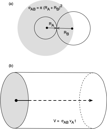
The kinetic theory of gases treats a gas as a large number of particles which are small compared to the distance between them. They are assumed to be in constant motion, with the full mass of each particle located at a point that is moving in space. Each kind of molecule has its own collision radius. Beyond their collision radii, the molecules exert no forces on each other, but when the distance between two molecules equals the sum of those molecules’ collision radii, they exert an infinite repulsive force on each other. This is commonly described by saying the molecules behave as hard spheres when they collide, but there is a significant difference. Hard spheres can have angular momentum due to spin, and they can transfer angular momentum when they collide. In the kinetic theory of gases, the mass of the molecules is all located at a point, so they cannot have angular momentum. Collisions between molecules are assumed to be perfectly elastic. This means that when two gas molecules collide there is no change in the total translational kinetic energy. As Figure F.1 (a) shows, an A molecule and a B molecule will collide when the distance between their centers equals the sum of their collision radii.

Figure F.1: Collisions According to the Kinetic Theory of Gases (a) Two point masses collide when the distance between them equals the sum of their collision radii. (b) As one point mass travels through space, it sweeps out a cylindrical volume.

F.2 The Boltzmann Distribution

As the name implies, the basic assumption of collision theory is that reaction takes place as a result of collisions between molecules. The development of collision theory begins with the Boltzmann distribution (sometimes called the Maxwell-Boltzmann distribution) which describes how available energy is distributed within a collection of molecules. For a gas at a given temperature, the Boltzmann distribution tells how many molecules will have a velocity, \(u\), which lies in the interval from \(u\) to \(u + du\). For a system which contains both A molecules and B molecules, a Boltzmann distribution of the velocities of A molecules, relative to one B molecule, is given in Equation F.1. The reduced mass, \(\mu\), that appears in the Boltzmann distribution is defined in Equation F.2.

\[ dN_A = \left(4\pi N_A^*u^2\right)\left(\frac{\mu}{2\pi k_BT}\right)^{3/2} \exp{\left(\frac{-\mu u^2}{2k_BT}\right)}du \tag{F.1}\]

\[ \mu = \frac{m_Am_B}{m_A + m_B} \tag{F.2}\]

F.3 Collision Theory

The kinetic theory of gases doesn’t include any attractive or repulsive forces between molecules except at the instant they collide. As a consequence, when an A molecule travels through space (between collisions) its center traces out a straight line (not a curve). This straight line can be used as the axis of a cylinder with a radius equal to the sum of the collision radii of an A molecule and a B molecule, Figure F.1 (b). Thus as the A molecule travels through space it sweeps out a cylindrical volume and a collision will occur if a B molecule has its center within this cylinder. The cross-sectional area of this cylinder is called the collision cross-section, \(\sigma_{AB}\). The collision cross section is calculated using Equation F.3.

\[ \sigma _{AB}=\pi \left(R_A + R_B\right)^2 \tag{F.3}\]

It is next assumed that B molecules are uniformly distributed throughout space. If \(N_B^*\) equals the number of B molecules per unit volume, then on average, there will be one B molecule in a volume, \(V_B^*\), as given by Equation F.4.

\[ V_B^* = \frac{1}{N_B^*} \tag{F.4}\]

The cylindrical volume swept out by a single A molecule before it collides with a B molecule will equal \(V_B^*\). The distance, \(L\), traveled by the A molecule before it undergoes collision can then be found using the formula for the volume of a cylinder, Equation F.5.

\[ L=\frac{V_B^*}{\sigma _{AB}} \tag{F.5}\]

The amount of time, \(t\), it takes the A molecule to travel the distance \(L\) can be found from its velocity, \(u\), relative to the B molecule with which it collides using Equation F.6 which is a simple rearrangement of the definition of a velocity.

\[ t=\frac{L}{u} \tag{F.6}\]

Thus, Equation F.6 can be used to find how long it takes, on average, for an A molecule to collide with a single B molecule. Substituting Equation F.5 into Equation F.6 leads to Equation F.7 for the amount of time, \(t_{\text{single}}\), required for an A molecule to have a single collision with a B molecule.

\[ t_{\text{single}}=\frac{V_B^*}{u\sigma _{AB}} \tag{F.7}\]

The time calculated using Equation F.7 is the period of the collisions of the A molecule with B molecules. The frequency of collisions of a single A molecule with a B molecule is equal to the reciprocal of this period. This frequency is only for collisions between the single A molecule under consideration and a B molecule. If \(\nu\) is used to represent frequency, the frequency of collisions of a single A molecule moving with a velocity, \(u\), is then given by Equation F.8.

\[ \nu_{\text{single,u}} = \frac{u\sigma _{AB}}{V_B^*} \tag{F.8}\]

The frequency of collisions involving all A molecules that are moving with one particular velocity, \(u\), is found by multiplying the frequency of collisions for a single A molecule by the total number of A molecules that are moving with that velocity, Equation F.9.

\[ \begin{pmatrix}\text{frequency of collisions}\\\text{involving all A molecules}\\\text{that have a velocity of } u \end{pmatrix} = \begin{pmatrix}\text{frequency of collisions}\\\text{of a single A molecule}\\\text{that has a velocity of } u \end{pmatrix}\begin{pmatrix}\text{number of A}\\\text{molecules that}\\\text{have a velocity of } u \end{pmatrix} \]

\[ \nu_{\text{all,u}} = \frac{u\sigma _{AB}}{V_B^*}dN_A^* \tag{F.9}\]

The frequency of all collisions between A molecules and B molecules (i. e. with any velocity) is found by summing Equation F.9 over all possible velocities. To do this, the Boltzmann distribution function, Equation F.1, is substituted into Equation F.9 along with substitution of Equation F.4. Since the velocity distribution is continuous, the summation takes the form of an integral over all possible velocities. The frequency of all collisions between A and B molecules is often called a collision number. The symbol \(Z_{AB}^{\prime}\) is used here to represent the frequency of all collisions between A molecules and B molecules, Equation F.10.

\[ Z_{AB}^{\prime}=\sum_u \nu_{\text{all,u}} = \sum_u \left(\frac{u\sigma _{AB}}{V_B^*}dN_A^*\right) \]

\[ Z_{AB}^{\prime}=\int_{u=0}^{u=\infty}\left(4\pi N_A^*N_B^*u^3\sigma _{AB}\right)\left(\frac{\mu}{2\pi k_BT}\right)^{3/2}\exp{\left(\frac{-\mu u^2}{2k_BT}\right)}du \]

\[ Z_{AB}^{\prime}=N_A^*N_B^*\sigma _{AB}\sqrt{\frac{8k_BT}{\pi \mu}} \tag{F.10}\]

Some of the collisions between the A molecules and the B molecules will involve very small relative velocities along the centerline between the molecules. These are cases that involve a glancing collision. Therefore, it is next assumed that there must be some minimum relative velocity along the centerline between the molecules if a collision is going to lead to reaction. Collisions which have at least this minimum velocity associated with them can be called reactive collisions, and their frequency can be represented by \(Z_{AB}\) (no prime). The frequency of collisions involving a velocity equal to or greater than some minimum, \(u_0\), can be found by replacing the lower limit of the integral above with \(u_0\), leading to Equation F.11 for \(Z_{AB}\), where \(\epsilon_0\) is the energy corresponding to the relative velocity, \(u_0\).

\[ Z_{AB}=N_A^*N_B^*\sigma _{AB}\sqrt{\frac{8k_BT}{\pi \mu}}\exp{\left(\frac{-\epsilon_0}{k_BT}\right)} \tag{F.11}\]

An analysis similar to the one just presented can be done for collisions between two A molecules. The primary difference is that one must be careful not to double-count the collisions. The resulting expression for the reactive collision frequency, \(Z_{AA}\), is given in Equation F.12. The analysis of a collision between three molecules, A, B, and C, requires a slight modification. The probability that all three molecules are in contact simultaneously is extremely small. Therefore, a collision is considered to have occurred whenever the centers of all three molecules are within a distance \(l\) of each other. The resulting expression for the reactive three-body collision frequency, \(Z_{ABC}\), is given in Equation F.13.

\[ Z_{AA}=\left(N_A^*\right)\sigma _{AA}\sqrt{\frac{2k_BT}{\pi \mu}}\exp{\left(\frac{-\epsilon_0}{k_BT}\right)} \tag{F.12}\]

\[ Z_{ABC}=8N_A^*N_B^*N_C^*\sigma _{AB}\sigma _{BC}l\sqrt{\frac{2k_BT}{\pi}}\left( \frac{1}{\mu_{AB}} -\frac{1}{\mu_{BC}} \right)\exp{\left(\frac{-\epsilon_0}{k_BT}\right)} \tag{F.13}\]

To this point, all the equations have been developed on the basis of molecules. Through the use of Avogadro’s number, \(N_{Av}\), each quantity appearing in the equations above can be converted to molar units.

\[ \epsilon_0 = \frac{E}{N_{Av}} \]

\[ k_B = \frac{R}{N_{Av}} \]

\[ N_i^*= N_{Av}C_i \]

\[ Z_{AB}= N_{Av}r_{j,f} \]

Substituting into Equations F.11, F.12 and F.13 gives Equations F.14, F.15 and F.16 for the generalized forward rates of bimolecular A-B reactions, bimolecular A-A reactions, and termolecular A-B-C reactions, respectively. It should be noted that these expressions only give the rate of the reaction in the forward direction, as indicated by the \(f\) appended to the subscript on the rate, \(r\).

\[ r_{AB,f}=N_{Av}\sigma _{AB}C_AC_B\sqrt{\frac{8k_BT}{\pi \mu}}\exp{\left(\frac{-E_j}{RT}\right)} \tag{F.14}\]

\[ r_{AA,f}=N_{Av}\sigma _{AA}C_A^2\sqrt{\frac{2k_BT}{\pi \mu}}\exp{\left(\frac{-E_j}{RT}\right)} \tag{F.15}\]

\[ \begin{align} r_{ABC,f} &= 8N_{Av}\sigma _{AB}\sigma _{BC}IC_AC_BC_C\sqrt{\frac{2k_BT}{\pi}} \\ & \times \left( \frac{1}{\mu_{AB}} -\frac{1}{\mu_{BC}} \right)\exp{\left(\frac{-E_j}{RT}\right)} \end{align} \tag{F.16}\]

Real molecules are not spheres. For an asymmetrical molecule, it may be necessary for the collision to take place in one part of the molecule in order to have reaction take place. If the colliding molecules are not oriented properly, necessary bonds can’t form and reaction can’t occur. The collision theory does not account for this kind of steric (geometric) limitation. If a reaction does have steric limitations, a constant is introduced into the rate expressions above. This constant, called a steric factor, is equal to the fraction of the collisions that have the orientation necessary for reaction to take place.

If the constants in the rate expressions above are unknown, they can be treated as adjustable parameters that are used to fit the rate expression to experimental data. In order to do so, groups of constants in the expressions above must be lumped together into single constants. Doing results in a single collision theory rate expression for the forward rate of an elementary reaction, Equation F.17, irrespective of whether it is a bimolecular A-B reaction, a bimolecular A-A reaction or a termolecular A-B-C reaction. Note that the stoichiometric coefficients of the reactants in that equation, \(\nu_{i,j}\), are negative numbers so the resulting exponents on the concentrations are positive.

\[ r_{j,f} = k_{0,j,f}\sqrt{T}\exp{\left(\frac{-E_{j,f}}{RT}\right)}\prod_{i_r} C_{i_r}^{-\nu_{i_u,j}} \tag{F.17}\]

Generally the net rate of reaction is more useful than the rate in the forward direction only. It is straightforward to generate an expression for the net rate of reaction. The definition of forward and reverse is completely arbitrary, so Equation F.17 can be used to generate an expression for the rate in the reverse direction, too.

\[ r_{j,r} = k_{0,j,r}\sqrt{T}\exp{\left(\frac{-E_{j,r}}{RT}\right)}\prod_{i_p} C_{i_p}^{\nu_{i_p,j}} \tag{F.18}\]

When the reaction reaches thermodynamic equilibrium, its net rate will equal zero, and as a consequence, the rate in the forward direction will equal the rate in the reverse direction. Thus, the two uni-directional rates can be set equal to each other while simultaneously recognizing that this is true only when the concentrations are equal to the equilibrium concentrations. Rearrangement of the resulting equation reveals that the ratio of the forward to the reverse rate coefficients must equal the concentration equilibrium constant for the elementary reaction, Equation F.19.

\[ r_{j,f}\Bigr\rvert_\text{equilibrium} = r_{j,r}\Bigr\rvert_\text{equilibrium} \]

\[ k_{0,j,f}\sqrt{T}\exp{\left(\frac{-E_{j,f}}{RT}\right)}\prod_{i_r} C_{i_r}^{-\nu_{i_r,j}} =k_{0,j,r}\sqrt{T}\exp{\left(\frac{-E_{j,r}}{RT}\right)}\prod_{i_p} C_{i_p,eq}^{\nu_{i_p,j}} \]

\[ \frac{k_{0,j,f}\sqrt{T}\exp{\left(\frac{-E_{j,f}}{RT}\right)}}{k_{0,j,r}\sqrt{T}\exp{\left(\frac{-E_{j,r}}{RT}\right)}} = \prod_i C_{i,eq}^{\nu_{i,j}} \]

\[ \frac{k_{0,j,f}\sqrt{T}\exp{\left(\frac{-E_{j,f}}{RT}\right)}}{k_{0,j,r}\sqrt{T}\exp{\left(\frac{-E_{j,r}}{RT}\right)}} = K_{j,eq_c} \tag{F.19}\]

An expression for the net rate of reaction according to collision theory is found by taking the difference between the forward and reverse rates. This can be written using the reverse rate coefficient, as in Equation F.20 or using the equilibrium constant, as in Equation F.21. The two forms are equivalent.

\[ r_j = r_{j,f} - r_{j,r} \]

\[ \begin{align} r_j &= k_{0,j,f}\sqrt{T}\exp{\left(\frac{-E_{j,f}}{RT}\right)}\prod_{i_r} C_{i_r}^{-\nu_{i_r,j}} \\&- k_{0,j,r}\sqrt{T}\exp{\left(\frac{-E_{j,r}}{RT}\right)}\prod_{i_p} C_{i_p}^{\nu_{i_p,j}} \end{align} \tag{F.20}\]

\[ r_j = k_{0,j,f}\sqrt{T}\exp{\left(\frac{-E_{j,f}}{RT}\right)}\left(\prod_{i_r} C_{i_r}^{-\nu_{i_r,j}}\right)\left(1-\frac{\displaystyle \prod_i C_i^{\nu_{i,j}}}{K_{j,eq_c}}\right) \tag{F.21}\]

It is often convenient to use partial pressures as the composition variables in a gas phase reaction system. Equations F.20 and F.21 can be easily converted so that partial pressures replace the concentrations. Since Equations F.20 and F.21 were derived assuming ideal gas type behavior, the concentrations and partial pressures are simply related via the ideal gas law, Equation F.22. Substitution of Equation F.22 into Equation F.20 or F.21 leads, in a straightforward manner, to a rate expression in terms of partial pressures instead of concentrations.

\[ C_i=\frac{n_i}{V}=\frac{P_i}{RT} \tag{F.22}\]

F.4 Limitations of Collision Theory

Collision theory as presented here is sometimes referred to as simple collision theory. It offers a simple molecular view of how reactions take place, and it can be useful for making rough approximations of the values of pre-exponential factors. There are several shortcomings of simple collision theory. First, the point-mass assumption is very limiting; it ignores internal motions within molecules and the energy associated with those internal motions. A second shortcoming is the absence of attractive and repulsive forces between molecules. In a real system, a molecule that is passing close to a second molecule may be attracted by it, causing it to travel in a curved path and collide with that molecule instead of continuing past it on a straight line path. Another shortcoming is the absence of orientation requirements for reaction to occur. Simple collision theory does not offer an easy way to estimate the activation energy, and it strictly applies only to gas phase reactions. There are also reactions for which the observed rate is higher than that predicted by the collision theory, and this can’t be explained by steric effects because they should lower the reaction rate, not raise it. There are more advanced formulations of collision theory that address the shortcomings enumerated here. Since these advanced formulations use more accurate representations of the molecules, they are often referred to as molecular reaction dynamics models.

F.5 Symbols Used in this Appendix

Symbol	Meaning
\(i\)	As subscript denotes one specific reagent present in the system. As a summation or continuous product index, indexes all reagents present in the system
\(i_p\)	As a subscript, denotes a specific reagent that is a product in the reaction under consideration. As a summation or continuous product index, indexes all reagents present in the system that are products in the reaction under consideration.
\(i_r\)	As a subscript, denotes a specific reagent that is a reactant in the reaction under consideration. As a summation or continuous product index, indexes all reagents present in the system that are reactants in the reaction under consideration.
\(j\)	subscript denoting one particular reaction occurring in the system.
\(k_{0,j,f}\)	Collision theory pre-exponential factor for reaction \(j\) in the forward direction; replacing \(f\) with \(r\) indicates reaction in the reverse direction.
\(k_B\)	Boltzmann constant.
\(l\)	Distance between centers of three molecules that corresponds to a three-body collision.
\(m_i\)	Mass of reagent \(i\).
\(n_i\)	Moles of reagent \(i\).
\(r_j\)	Net rate of reaction \(j\); an additional subscripted \(f\) or \(r\) indicates reaction in the forward or reverse direction.
\(r_{AB,f}\)	Forward rate of bimolecular reaction of reagents A and B; AA denotes bimolecular reaction of two A molecules and ABC denotes termolecular reaction of A, B and C.
\(t\)	Average time between collisions.
\(t_{\text{single}}\)	Time required for a single collision of an A molecule with a B molecule.
\(u\)	As a variable, velocity. As a subscript, denotes one specific velocity. As a summation or continuous product index, indexes all possible velocities.
\(C_i\)	Molar concentration of reagent \(i\); an additional subscripted \(eq\) indicates equilibrium concentration.
\(E\)	Collision energy per mole.
\(E_j\)	Activation energy for reaction \(j\); an additional subscripted \(f\) or \(r\) indicates reaction in the forward or reverse direction.
\(K_{j,eq_c}\)	Concentration equilibrium constant for reaction \(j\).
\(L\)	Average distance a molecule travels between collisions.
\(N_{Av}\)	Avogadro’s number.
\(N_i\)	Number of molecules of reagent \(i\).
\(N_i^*\)	Number of molecules of reagent \(i\) per volume.
\(P_i\)	Partial pressure of reagent \(i\).
\(R\)	Ideal gas constant.
\(R_i\)	Collision radius for a molecule of reagent \(i\).
\(T\)	Temperature.
\(V\)	Volume.
\(V_i^*\)	Volume per molecule of reagent \(i\).
\(Z_{AB}\)	Frequency of collisions between A molecules and B molecules with an energy above some threshold, \(\epsilon _0\); AA denotes collision of two A molecules and ABC denotes three-bodied collisions involving A, B and C.
\(Z_{AB}^{\prime}\)	Frequency of all collisions between A molecules and B molecules.
\(\epsilon _0\)	Collision energy per molecule.
\(\mu\)	Reduced mass.
\(\nu_{\text{all,u}}\)	Frequency of collisions of all A molecules moving with velocity, \(u\).
\(\nu_{\text{single,u}}\)	Frequency of collisions of a single A molecule moving with velocity, \(u\).
\(\sigma _{AB}\)	Cross-section for collision between an A and a B molecule.