16 Thermally Back-Mixed PFRs
In a PFR the composition and temperature vary continuously from the inlet to the outlet. When an exothermic reaction is taking place in an adiabatic PFR, the temperature equals the feed temperature at the inlet and continuously increases until it reaches the outlet temperature at the end of the reactor. In a thermally backmixed PFR, some of the heat released by the reaction is transferred to the feed entering the reactor. This is beneficial because the rate of most reactions increases with temperature.
16.1 Thermally Backmixed PFRs
When a typical exothermic reaction takes place in an adiabatic reactor, either a CSTR or a PFR, two competing effects are present. As the reaction proceeds, the temperature increases (a favorable effect, tending to increase the reaction rate) and the reactant concentration decreases (an unfavorable effect, tending to decrease the reaction rate). In many cases, the temperature effect predominates at lower conversions and the reactant concentration effect predominates at higher conversions. In a PFR, the reactant concentration decreases gradusec-ideal_pfr_eqnsally (favorable behavior since it tends to keep the rate as high as possible), but the temperature also increases gradually (unfavorable behavior since the rate coefficient increases gradually). In a CSTR, the reactant concentration is low (equal to the final value) for the entire time the fluid reacts (unfavorable behavior since it tends to make the rate low), but the temperature is at its highest value throughout the time the fluid reacts (favorable behavior since it tends to make the rate high). Thus, neither a single CSTR nor a single PFR is ideally suited to an exothermic reaction.
In Chapter 15, it was shown that using a cascade of CSTRs makes the CSTRs behave a little more like a PFR. Here, it will be seen that by augmenting a PFR with a heat exchanger, it is sometimes possible to impart CSTR-like thermal behavior to a PFR while retaining PFR-like behavior with respect to the composition. To see how this can be accomplished, examine Figure 16.1 which shows a heat exchanger connected to a PFR. There are two compartments in the heat exchange; the feed flows through one compartment and the product stream from the PFR flows through the other. The two compartments are physically separated by a wall (red), so there is no mass exchanged between the streams. However, it is possible for heat to be conducted through the (red) wall. In this way, as the feed flows through the lower compartment of the heat exchanger, heat is transferred to it from the PFR product stream flowing through the upper compartment. This is similar to what happens thermally in a CSTR where the complete back-mixing in the CSTR immediately heats the feed to the final outlet temperature. Due to the heat exchanger in Figure 16.1, the PFR inlet temperature is higher and consequently, the rate at the PFR inlet is larger than it would be without the heat exchanger.
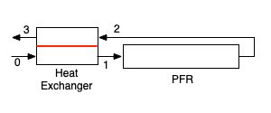
When a thermally backmixed PFR is used, it is sometimes possible for an exothermic reaction to occur auto-thermally. That is, with the heat exchanger the reaction can reach a high steady state conversion without the need to continually supply heat from another source. In contrast, the steady state conversion could be much, much lower without the heat exchanger. In particular, consider a situation where the feed, stream 0, is supplied at a temperature where the rate of reaction is very small. If this feed is admitted directly to the reactor, without a heat exchanger, very little reaction will occur and consequently very little heat of reaction will be released. As a result, the temperature will not rise significantly, and so the rate will remain small through the entire reactor. If the same feed is used, but it first passes through a heat exchanger as in Figure 16.1, the feed will enter the reactor at a higher temperature where the rate is high enough to cause some reaction to occur. That, in turn will release more heat so that the rate is appreciable throughout the reactor. Of course, as the reactant is depleted, the rate will eventually decrease. Nonetheless, for a typical exothermic reaction taking place adiabatically, a thermally backmixed PFR like that shown in Figure 16.1 offers the best features of both a CSTR and a PFR: the feed is immediately heated, as in a CSTR, while the reactant concentration starts high and decreases gradually, as in a PFR.
16.2 Analysis of Thermally Backmixed PFRs
In order to analyze a thermally backmixed PFR, the design equations must be generated for the PFR and the heat exchanger. Here only steady state operation will be considered. The reactor design equations for a steady-state PFR, Equations 6.39 and 6.40, were derived in Appendix E.5, presented in [Chapter -sec-ideal_pfr_eqns@sec-ideal_pfr_eqns], and discussed in Chapter 13. The general mole and reacting fluid energy balances are reproduced below. Recall that these equations also can be written using the reactor volume as the dependent variable, and the sensible heat term can be written in terms of the volumetric or gravimetric heat capacity of the reacting fluid as a whole. If the PFR is heated or cooled using a heat exchange fluid, and energy balance on that fluid, Equation 6.2 or Equation 6.6, as appropriate, must be added to the reactor design equations, and if there is pressure drop a momentum balance, Equation 6.41 or Equation 6.42, as appropriate, must be added.
\[ \frac{d \dot{n}_i}{d z} =\frac{\pi D^2}{4}\sum_j \nu_{i,j}r_j \]
\[ \left(\sum_i \dot{n}_i \hat{C}_{p,i} \right) \frac{d T}{d z} = \pi D U\left( T_{ex} - T \right) - \frac{\pi D^2}{4}\sum_j r_j \Delta H_j \]
The design equations for a counter-current heat exchanger like that depicted in Figure 16.1 were presented in Chapter 15. Only a brief re-cap is offered here. In terms of Figure 16.1, stream 1 in the equations is the stream that enters the heat exchanger as stream 0 and leaves as stream 1 and stream 2 enters the heat exchanger as stream 2 and leaves as stream 3. Thus, the mole balances are trivial, and assuming no heat loss from the heat eachanger, the energy balance requires that the heat gained by the feed must equal the heat lost by the stream leaving the reactor as it passes through the heat exchanger. The sensible heats in the energy balance instead can be expressed in terms of the volumetric or gravimetric heat capacity of the reacting fluid as a whole, when appropriate.
\[ 0 = \dot{n}_{i,0} - \dot{n}_{i,1} \]
\[ 0 = \dot{n}_{i,2} - \dot{n}_{i,3} \]
\[ \sum_i \left( \dot{n}_{i,0} \int_{T_0}^{T_1}\hat{C}_{p,i} dT\right) = \sum_i \left( \dot{n}_{i,2} \int_{T_3}^{T_2}\hat{C}_{p,i} dT\right) \]
The rate of heat transfer can also be set equal to the rate at which the feed gains heat.
\[ \sum_i \left( \dot{n}_{i,0} \int_{T_0}^{T_1}\hat{C}_{p,i} dT\right) = U_{LM}A \Delta T_{LM} \]
\[ \sum_i \left( \dot{n}_{i,0} \int_{T_0}^{T_1}\hat{C}_{p,i} dT\right) = U_{AM}A \Delta T_{AM} \]
\[ \Delta T_{LM} = \frac{\left(T_3 - T_0\right) - \left( T_2 - T_1 \right)}{\ln{\left(\displaystyle\frac{T_3 - T_0}{T_2 - T_1 }\right)}} \]
\[ \Delta T_{AM} = \frac{\left(T_3 - T_0\right) + \left(T_2 - T_1\right)}{2} \]
Alternatively, when analyzing a thermally backmixed PFR the cold approach, Equation 16.1, is sometimes specified instead of the heat transfer coefficient and area.
\[ \Delta T_{cold} = T_3 - T_0 \tag{16.1}\]
A key point associated with the heat exchanger is that the two fluid streams do not mix. It should also be noted that the equations presented here are for a counter-current flow. Many other styles of heat exchanger might be used, in which case a good reference on heat transfer should be consulted. The focus here is on the reactor and reaction, not the details of the heat exchanger.
16.2.1 Solving the Thermally Backmixed PFR Design Equations
Most commonly with a system like that shown in Figure 16.1, the composition of the feed, stream 0, is known, and consequently, the composition of stream 1, but not its temperature, is also known. One of the four temperatures will also be known (commonly \(T_0\)). In many cases, it won’t be possible to solve the PFR design equations independently because \(T_1\) will not be known. In that situation, the reactor design equations for the PFR and the mole and energy balances for the heat exchanger must be solved simultaneously. The PFR design equations are IVODEs while the heat exchanger balance equations are ATEs.
Together, the reactor and heat exchanger balances constitute a set of differential-algebraic equations (DAEs). When they must be solved numerically, the mathematical formulation of the solution is different from solving sets of ATEs or sets of IVODEs. Appendix F.5.3 describes the numerical solution of DAEs of this type in some detail. Essentially, the formulation begins with the ATE heat exchanger balances. The critical element of the formulation is that the temperature of stream 1 must be one of the unknowns to be found by solving the heat exchanger balances, and stream 2 must not be one of the unknowns. When that is the case, the PFR design equations can be solved within the function that evaluates the residuals for the heat exchanger balances. Again, see Appendix F.5.3 for a more detailed description.
16.2.2 Multiplicity of Thermally Backmixed PFR Steady States
Chapter 12.5 showed that for a CSTR with a fixed set of operating parameters there may be more than one steady state. Without going into the mathematical details, when there is backmixing in a reactor, multiple steady states may occur. Put differently, when the input to a reactor can be affected by the output from that reactor, multiple steady states may be observed. In a thermally backmixed PFR, the input and output flow streams exchange energy. Consequently, the inlet temperature of a thermally backmixed PFR temperature is affected by its outlet temperature. All that to say that multiple steady states are possible in thermally back-mixed PFRs. The discussion following Example 16.3.2 considers the steady-state multiplicity of thermally backmixed PFRs in greater detail.
16.3 Examples
This chapter presents two examples of the analysis of a thermally backmixed PFR. The first example illustrates a simple response assignment where the conversion is specified and the reactor volume must be determined by solving the reactor design equations and the heat exchanger balances simultaneously. In the second example, where the reactor volume is known and the final composition must be determined, multiple steady states exist.
16.3.1 Determining the Volume of a Thermally Backmixed PFR for a Specified Conversion.
Reaction (1) takes place in an adiabatic, steady state PFR using 750 dm3 min-1 of a constant-density liquid solution containing the reactant at a concentration of 3.8 mol dm-3 and a temperature of 25 °C. Pressure drop in the reactor is neglibible. The heat of reaction is -79.8 kJ mol-1, and may be assumed to be constant over the range of temperatures where this reactor operates. The heat capacity of the solution is equal to 987 cal L-1 K-1, independent of composition and temperature. For a conversion of 80%, compare the required PFR volume without thermal backmixing to that with thermal backmixing, assuming a simple counter-current heat exchanger with ULMA = 1500 kJ min-1 K-1. The rate is first order in the concentration of A, the Arrhenius pre-exponential factor is 3.38 x 10⁶ min-1, and the activation energy is 50 kJ mol-1.
\[ A \rightarrow Z \tag{1} \]
I will begin by sketching the reactor system and summarizing the assignment. The system consists of a thermally backmixed PFR like that in Figure 16.1. I can use the stream labels as subscripts on variables to show the stream to which they apply.
16.3.1.1 Assignment Summary
Reactor System Schematic:
Given and Known Constants: \(\dot{V}_0\) = 750 dm3 min-1, \(C_{A,0}\) = 3.8 mol dm-3, \(T_0\) = 25 °C, \(\Delta H_1\) = -79.8 kJ mol-1, \(\breve{C}_p\) = 987 cal L-1 K-1, \(f_A\) = 80%, \(U_{LM}A\) = 1500 kJ min-1 K-1, \(k_{0,1}\) = 3.38 x 10⁶ min-1, \(E_1\) = 50 kJ mol-1, \(R\) = 8.314 x 10⁻³ kJ mol-1 K-1.
Reactor System: Adiabatic, steady-state PFR with and without thermal backmixing.
Quantities of Interest: \(V_{PFR}\) with and without thermal backmixing.
16.3.1.2 Mathematical Formulation of the Solution
There are two pieces of equipment in the reactor system: the PFR and the heat exchanger. If I’m going to model the system, I’ll need to write the reactor design equations for the PFR and for the heat exchanger. I’ll start with the PFR design equations. There isn’t an exchange fluid to write an energy balance for, and pressure drop is negligible, so the reactor design equations consist of mole balances on each reagent and an energy balance on the reacting fluid. The reactor operates at steady state, so the general form of the mole balance is given in Equation 6.39.
\[ \frac{d \dot{n}_i}{d z} =\frac{\pi D^2}{4}\sum_j \nu_{i,j}r_j \]
The assignment asks for the reactor volume, and I don’t need the length and diameter separately because there isn’t any heat transfer through the wall of the PFR, so I can rewrite the mole balance using the volume as the independent variable. At the same time, I can expand the summation over the reactions to a single term for the one reaction that is taking place.
\[ \frac{d \dot{n}_i}{\frac{\pi D^2}{4}dz} = \frac{d \dot{n}_i}{dV} = \nu_{i,1}r_1 \]
The general form of the steady-state PFR energy balance is given in Equation 6.40. Here, too, the balance can be rewritten using the volume as the independent variable, and the summation over the reactions can be expanded to a single term for the one reaction that is occurring. The reactor operates adiabatically, so the heat transfer term is equal to zero. The assignment provides the volumetric heat capacity, so the sensible heat term can be written in terms of it. Finally, I can rearrange the equation into the form of a derivative expression.
\[ \cancelto{\dot{V}\breve{C}_p}{\left(\sum_i \dot{n}_i \hat{C}_{p,i} \right)} \frac{dT}{dz} = \cancelto{0}{\pi D U\left( T_{ex} - T \right)} - \frac{\pi D^2}{4}\sum_j r_j \Delta H_j \]
\[ \frac{dT}{\frac{\pi D^2}{4}dz} = \frac{dT}{dV} = - \frac{r_1 \Delta H_1}{\dot{V}\breve{C}_p} \]
Reactor Design Equations
Mole balance design equations on A and Z in the PFR are presented in equations (2) and (3), and an energy balance on the reacting fluid is given in equation (4).
\[ \frac{d \dot{n}_A}{dV} = -r_1 \tag{2} \]
\[ \frac{d \dot{n}_Z}{dV} = r_1 \tag{3} \]
\[ \frac{dT}{dV} = - \frac{r_1 \Delta H_1}{\dot{V}\breve{C}_p} \tag{4} \]
The PFR reactor design equations are IVODEs, and the number of dependent variables (three: \(\dot{n}_A\), \(\dot{n}_Z\), and \(T\)) is equal to the number of equations. That means I don’t need to add an equation or eliminate a dependent variable, but I do need to specify initial values and a stopping criterion. Here I can define \(V=0\) to be the PFR inlet, in which case the initial values are simply the values of the dependent variables at the reactor inlet.
In this example, the feed does not contain reagent Z, and since there isn’t any fluid mixing in the heat exchanger, the molar flow rate of Z in stream 1 will also equal zero. Similarly, the molar flow rate of reagent A in stream 1 will equal its flow rate in stream 0. Knowing that along with the fractional conversion of A, I can calculate the outlet molar flow rate of A and use it as the stopping criterion.
Initial Values and Stopping Criterion
| Variable | Initial Value | Stopping Criterion |
|---|---|---|
| \(V\) | \(0\) | |
| \(\dot{n}_A\) | \(\dot{n}_{A,1}\) | \(\dot{n}_{A,2}\) |
| \(\dot{n}_Z\) | \(0\) | |
| \(T\) | \(T_1\) |
I also need mole and energy balances on the heat exchanger. The mole balances are trivial. I can write an energy balance that requires the heat gained by the feed as it flows from 0 to 1 must equal the heat lost by the converted fluid as it flows 2 to 3 in the schematic. I am given the volumetric heat capacity, so I’ll express those energies using it, and I’ll write the equation in the form of a resitual expression. I can also note that the reacting fluid is a liquid, so assuming it to be an ideal, incompressible mixture, the volumetric flow rate of streams 0, 1, 2, and 3 are all equal.
\[ \cancel{\dot{V}_0 \breve{C}_p} \left(T_1 - T_0 \right) = \cancel{\dot{V}_0 \breve{C}_p} \left(T_2 - T_3 \right) \qquad \Rightarrow \qquad 0 = \left(T_1 - T_0 \right) - \left(T_2 - T_3 \right) \]
I am given the heat transfer coefficient, so I can also write an expression for the rate of heat transfer and set it equal to the rate at which heat is transferred to the feed stream, again in the form of a residual expression.
\[ 0 =\dot{V}_0 \breve{C}_p \left(T_1 - T_0 \right) - U_{LM}A \Delta T_{LM} \]
I can substitute the defining equation for a log-mean temperature difference into that equation. However, in this system the volumetric flow rate and the heat capacity are constants. As a consequence \(T_3 - T_0\) will be equal to \(T_2 - T_1\). (This can be seen by rearranging the energy balance above.) As pointed out in Chapter 15, when this is true, the log-mean temperature difference becomes indeterminate, and should be set equal to either of the two temperature differences.
\[ \frac{\left(T_3 - T_0 \right) - \left(T_2 - T_1 \right)}{\ln \left( \frac{T_3 - T_0}{T_2 - T_1} \right)} \qquad \underset{T_3 - T_0 = T_2 - T_1}{\Rightarrow} \qquad T_3 - T_0 \]
\[ 0 = \dot{V}_0 \breve{C}_p \left(T_1 - T_0 \right) - U_{LM}A \left(T_3 - T_0\right) \]
Heat Exchanger Design Equations
\[ \dot{n}_{A,0} = \dot{n}_{A,1} \tag{5} \]
\[ \dot{n}_{Z,0} = \dot{n}_{Z,1} \tag{6} \]
\[ \dot{n}_{A,2} = \dot{n}_{A,3} \tag{7} \]
\[ \dot{n}_{Z,2} = \dot{n}_{Z,3} \tag{8} \]
\[ 0 = \left(T_1 - T_0 \right) - \left(T_2 - T_3 \right) = \epsilon_1 \tag{9} \]
\[ 0 = \dot{V}_0 \breve{C}_p \left(T_1 - T_0 \right) - U_{LM}A \left(T_3 - T_0\right) = \epsilon_2 \tag{10} \]
There are two heat exchanger design equations (9) and (10). That means I can solve them to find two unknown quantities. Examining those equations I see that they contain three unknown quantities: \(T_1\), \(T_2\), and \(T_3\). As described in Appendix F.5.3, I will solve the heat exchanger design equations, (9) and (10), for \(T_1\) and \(T_3\). To do so numerically, I will have to (a) provide an initial guess for those unknowns and (b) evaluate the residuals. At the point where I need to evaluate the residuals, I will have a guess for \(T_1\) and \(T_3\). So, to evaluate the residuals I’ll need to calculate any other unknown quantities that appear in them. In this case, the only other unknown is \(T_2\). \(T_1\) is one of the initial values I need for solving the PFR design equations, so using the guess for \(T_1\), I can solve the PFR design equations to find the outlet temperature, \(T_2\).
Ancillary Equations for Evaluating the Heat Exchanger Residuals
Solving the PFR design equations, (2) - (4), will yield the molar flow rates of A and Z and the temperature within the PFR.
\[ T_2 = T \big\vert_{V_{PFR}} \tag{11} \]
In order to solve the IVODEs numerically I’ll need to do two things: calculate the values of the derivatives at the start of each integration step and calculate all of the initial and final values in Table 16.1. At the start of each integration step, the independent variable \(V\) and dependent variables \(\dot{n}_A\), \(\dot{n}_Z\), and \(T\) will be known, as will the given and known constants listed in the assignment summary. I will need to calculate any other quantities that appear in the IVODE design equations (2) thorough (4).
Here, the only quantity I’ll need to calculate is the rate, \(r_1\). I’m told that the reaction is first order in the concentrations of A, so I can write the rate expression.
\[ r_1 = kC_A \]
Before I can evaluate the rate, I’ll need to calculate \(k\) and \(C_A\). The former I can do with the Arrhenius expression, Equation 4.8, and the latter with the definition of concentration for a flow system, Equation 2.15. I noted earlier that since the fluid is an incompressible liquid, each of the flow rates is equal to \(\dot{V}_0\).
Ancillary Equations for Evaluating the Derivatives
\[ r_1 = k_{0,1} \exp{\left( \frac{-E_1}{RT} \right)}\frac{\dot{n_A}}{\dot{V}_0} \tag{12} \]
When I solve the IVODEs numerically, I’ll also need to calculate the initial and final values in Table 16.1. I will be solving the IVODE from within the function that evaluates the residuals, equations (9) and (10). At that point a value for \(T_1\) will be available. The molar flow rate of A in the feed can be calculated using given information, and according to equation (5), that is equal to \(\dot{n}_{A,1}\). Knowing the inlet molar flow rate of A, I can then calculate it’s outlet molar flow rate from the specified conversion.
Ancillary Equations for Calculating the Initial and Final Values
\[ \dot{n}_{A,0} = \dot{V}_0 C_{A,0} = \dot{n}_{A,1} \tag{13} \]
\[ \dot{n}_{A,2} = \dot{n}_{A,1} \left( 1 - f_A \right) \tag{14} \]
At this point the heat exchanger design equations can be solved numerically for \(T_1\) and \(T_3\). Using the resulting value of \(T_1\), the PFR design equations can be solved numerically to get corresponding sets of values of \(V\), \(\dot{n}_A\), \(\dot{n}_Z\), and \(T\) spanning the range from their initial (inlet) values to their final (outlet) values. The outlet value of \(V\) is the requested PFR volume.
Ancillary Equations for Calculating the Quantities of Interest
Solving the heat exchanger design equations, (9) and (10), yields \(T_1\) and \(T_3\).Solving the reactor design equations using that value of \(T_1\) yields corresponding sets of values of \(V\), \(\dot{n}_A\), \(\dot{n}_Z\), and \(T\). The final value of \(V\) is the PFR volume.
Calculations Summary
- Substitute given and known constants into all equations.
- When it is necessary to evaluate the derivatives
- \(V\), \(\dot{n}_A\), \(\dot{n}_Z\), and \(T\) will be available.
- calculate \(r_1\) using equation (12).
- evaluate the derivatives, equations (2) - (4).
- When it is necessary to calculate the initial and final values in Table 16.1
- \(\dot{n}_{A,0}\) is a known constant.
- \(T_1\) will be available.
- calculate \(\dot{n}_{A,1}\) and \(\dot{n}_{A,2}\) using equations (13) and (14).
- When it is necessary to evaluate the residuals corresponding to equations (9) and (10).
- a guess for \(T_1\) and \(T_3\) will be available.
- solve the PFR design equations using the initial and final values in Table 16.1.
- calculate \(T_2\) using the results in equation (11).
- evaluate the residuals, \(\epsilon_1\) and \(\epsilon_2\), using equations (9) and (10).
- When it is necessary to calculate the quantities of interest, \(V_{PFR}\)
- corresponding sets of values of \(V\), \(\dot{n}_A\), \(\dot{n}_Z\), and \(T\), spanning the range from their initial values to their final values will be available.
- the final value of \(V\) is \(V_{PFR}\).
16.3.1.3 Numerical implementation of the Solution
- Make the given and known constants available for use in all functions.
- Write a derivatives function that
- receives the independent and dependent variables, \(V\), \(\dot{n}_A\), \(\dot{n}_Z\), and \(T\), as arguments, and
- evaluates the derivatives as described in step 2 of the calculations summary, and returns them.
- Write a reactor model function that
- receives the value of \(T_1\) as an argument
- calculates the initial and final values in Table 16.1 as described in step 3 of the calculations summary,
- gets corresponding sets of values of \(V\), \(\dot{n}_A\), \(\dot{n}_Z\), and \(T\), spanning the range from their initial values to their final values by calling an IVODE solver and passing the following information to it
- the initial values and stopping criterion in Table 16.1 and
- the name of the derivatives function from step 2 above,
- checks that the solver successfully solved the IVODEs, and
- returns the values returned by the IVODE solver.
- Write a residuals function that
- receives a guess for \(T_1\) and \(T_3\),
- evaluates the residual as described in step 4 of the calculations summary, and
- returns the values of \(\epsilon_1\) and \(\epsilon_2\).
- Perform the analysis by
- calling the reactor model function from step 3 above, passing \(T_0\) as an argument.
- the final value of \(V\) is the PFR volume without backmixing.
- setting an initial guess for \(T_1\) and \(T_3\)
- calculating \(T_1\) and \(T_3\) by calling an ATE solver, passing it the name of the residuals function from step 4 and the initial guess, and checking that the solver converged.
- calling the reactor model function from step 3 above, passing the value of \(T_1\) from the previous step as an argument.
- the final value of \(V\) is the PFR volume with backmixing.
- calling the reactor model function from step 3 above, passing \(T_0\) as an argument.
16.3.1.4 Results and Discussion
The calculations were performed as described above. Without thermal backmixing the PFR volume is 3.74 x 10⁴ L. When the PFR is thermally backmixed, its volume is 7.93 x 10³ L. The reason for the difference is easy to understand. The key in either case is the inlet temperature. A higher inlet temperature results in a larger rate coefficient, and therefore a larger rate, near the inlet to the reactor. When the rate is larger, the reacting fluid needs less time in the reactor to reach the final conversion. The time in the reactor is the reactor volume divided by the volumetric flow rate, so when the reacting fluid requires less time in the reactor, the volume is smaller since the volumetric flow rate is constant.
As discussed in Chapter 14, the rate may decrease steadily as the fluid passes through the reactor, or it may rise, reach a maximum and then decrease, but in either case, the rate a given distance into the reactor will always be greater if the feed enters at a higher temperature. In this particular system, the outlet temperature from the PFR without backmixing is 83.7 °C while that from the PFR with backmxing is 112 °C.
It was noted in this chapter that multiple steady states are possible in thermally backmixed PFRs. In this assignment, it wasn’t necessary to worry about that because the design equations were being solved to find a reactor operating parameter, namely the volume. The output here was fixed, and there will only be one volume that results in the specified conversion.
Multiplicity becomes important when the reactor operating parameters are fixed and the design equations are being solved to find the outlet flows and temperatures. Indeed, if a reactor with the volume found in this assignment was operated as described in this assignment, there is a possibility that more than one conversion might be observed if multiple steady states are possible. If that were true, one of the observed conversions would be the 80% specified in this assignment. Example 16.3.1 illustrates a situation where this is true and the discussion describes one way to determine whether multiple steady states are possible.
16.3.2 Conversion in a Thermally Backmixed PFR
An adiabatic PFR with a volume of 4 m3 will be used to process 1.25 mol s-1 of an equimolar gas phase mixture of A and B at 300 K and 2.5 atm. This feed will be pre-heated using the product stream from the reactor. The heat of reaction is constant and equal to -8,600 cal mol-1. The heat capacity of the gas is constant and equal to 25.8 cal mol-1 K-1. Pressure drop in the reactor is negligible. The heat transfer area multipled by the heat transfer coefficient UAMA = 13.6 cal K-1 s-1. What will the final conversion equal if reaction (1) takes place with a rate given by equation (2) with the pre-exponential factor equal to 8.12 x 10² s-1 and the activation energy equal to 9,500 cal mol-1.?
\[ A + B \rightarrow Y + Z \tag{1} \]
\[ r_1 = k_1 C_A \tag{2} \]
The system to be modeled in this assignment is a thermally backmixed PFR. I’ll start by sketching the system and labeling the flow streams. Then I will summarize the assignment, using the stream labels as subscripts when appropriate.
16.3.2.1 Assignment Summary
System Schematic
Given and Known Constants: \(V_{PFR}\) = 4 m3, \(\dot{n}_{total,0}\) = 1.25 mol s-1, \(y_{A,0}\) = 0.5, \(y_{B,0}\) = 0.5, \(T_0\) = 300 K, \(P\) = 2.5 atm, \(\Delta H_1\) = -8,600 cal mol-1, \(\hat{C}_p\) = 25.8 cal mol-1 K-1, \(U_{MA}A\) = 13.6 cal K-1 s-1, \(k_{0,1}\) = 8.12 x 10² s-1, \(E_1\) = 9,500 cal mol-1, \(R\) = 1.987 cal mol-1 K-1 = 8.206 x 10⁻⁵ m3 atm mol-1 K-1.
Reactor System: Adiabatic, thermally backmixed PFR
Quantities of Interest: \(f_A\)
16.3.2.2 Mathematical Formulation of the Solution
In order to model this system I’ll need design equations for the PFR and for the heat exchanger. The PFR is adiabatic with negligible pressure drop, so I don’t need an energy balance on the heat exchange fluid (since there isn’t one) or a momentum balance. I do need steady-state PFR mole balances and a steady-state PFR energy balance on the reacting fluid. The general form of the mole balance is given in Equation 6.39. I don’t have or need the reactor diameter and length, so I’ll rewrite the balance equations using the reactor volume as the independent variable. I’ll also expand the summation over the reactions; here there is only one reaction.
\[ \frac{d \dot{n}_i}{dz} = \frac{\pi D^2}{4}\sum_j \nu_{i,j}r_j \]
\[ \frac{d \dot{n}_i}{\frac{\pi D^2}{4}dz} = \frac{d \dot{n}_i}{dV} = \nu_{i,1}r_1 \]
The general form of the steady-state PFR energy balance is given in Equation 6.40. Here the heat transfer term goes to zero. I’ll rewrite it in the form of a derivative expression with the reactor volume as the independent variable and the summations expanded. The heat capacity given in this assignment is the overall molar heat capacity.
\[ \left(\sum_i \dot{n}_i \hat{C}_{p,i} \right) \frac{d T}{d z} = \cancelto{0}{\pi D U\left( T_{ex} - T \right)} - \frac{\pi D^2}{4}\sum_j r_j \Delta H_j \]
\[ \frac{d T}{\frac{\pi D^2}{4}dz} = \frac{d T}{dV} = \frac{-r_1 \Delta H_1}{\left( \dot{n}_{A} + \dot{n}_{B} + \dot{n}_{Y} + \dot{n}_{Z} + \right)\hat{C}_p} \]
Reactor Design Equations
PFR mole balance design equations for A, B, Y, and Z are presented in equations (3) through (6), and the energy balance on the reacting fluid is given in equation (7).
\[ \frac{d \dot{n}_A}{dV} = - r_1 \tag{3} \]
\[ \frac{d \dot{n}_B}{dV} = - r_1 \tag{4} \]
\[ \frac{d \dot{n}_Y}{dV} = r_1 \tag{5} \]
\[ \frac{d \dot{n}_Z}{dV} = r_1 \tag{6} \]
\[ \frac{d T}{dV} = \frac{-r_1 \Delta H_1}{\left( \dot{n}_{A} + \dot{n}_{B} + \dot{n}_{Y} + \dot{n}_{Z} \right)\hat{C}_p} \tag{7} \]
The PFR design equations are IVODEs. There are five equations and they contain five dependent variables (\(\dot{n}_A\),\(\dot{n}_B\), \(\dot{n}_Y\), \(\dot{n}_Z\), and \(T\)), so they can be solved. In order to do so numerically I’ll need initial values and a stopping criterion. I can define \(V=0\) as the reactor inlet. In that case the initial values are the values of the dependent variables in stream 1, the reactor inlet. I know the PFR volume, so I can use that as the stopping criterion. The feed only contains A and B, and nothing gets mixed into it before it enters the reactor, so the inlet molar flow rates of Y and Z are zero.
Initial Values and Stopping Criterion
| Variable | Initial Value | Stopping Criterion |
|---|---|---|
| \(V\) | \(0\) | \(V_{PFR}\) |
| \(\dot{n}_A\) | \(\dot{n}_{A,1}\) | |
| \(\dot{n}_B\) | \(\dot{n}_{B,1}\) | |
| \(\dot{n}_A\) | \(0\) | |
| \(\dot{n}_A\) | \(0\) | |
| \(T\) | \(T_1\) |
I also need design equations for the heat exchanger. The mole balances are trivial: the molar flow rates in stream 0 equal those in stream 1 and the molar flow rates in stream 2 equal those in stream 3. The energy balance simply requires the heat gained by stream 0 to equal the heat lost by stream 2. The expression for the rate of heat transfer simply requires the rate at which heat is transferred to equal the rate at which heat is gained by stream 0. The heat capacity is constant, making it easy to evaluate the integrals.
\[ \sum_i \left( \dot{n}_{i,0} \int_{T_0}^{T_1}\hat{C}_{p,i} dT\right) = \sum_i \left( \dot{n}_{i2} \int_{T_3}^{T_2}\hat{C}_{p,i} dT\right) \]
\[ 0 = \left( \dot{n}_{A,0} + \dot{n}_{B,0} + \dot{n}_{Y,0} + \dot{n}_{Z,0} \right)\cancel{\hat{C}_p}\left( T_1 - T_0 \right) - \left( \dot{n}_{A,2} + \dot{n}_{B,2} + \dot{n}_{Y,2} + \dot{n}_{Z,2} \right)\cancel{\hat{C}_p}\left( T_3 - T_2 \right) \]
The rate of heat transfer can also be set equal to the rate at which the feed gains heat.
\[ \sum_i \left( \dot{n}_{i,0} \int_{T_0}^{T_1}\hat{C}_{p,i} dT\right) = U_{AM}A \Delta T_{AM} \]
\[ 0 = \left( \dot{n}_{A,0} + \dot{n}_{B,0} + \dot{n}_{Y,0} + \dot{n}_{Z,0} \right)\hat{C}_p\left( T_1 - T_0 \right) - U_{AM}A \left(\frac{\left(T_3 - T_0\right) + \left(T_2 - T_1\right)}{2}\right) \]
Heat Exchanger Design Equations
\[ 0 = \dot{n}_{i,0} - \dot{n}_{i,1}; \qquad i = \text{ A, B, Y, and Z} \tag{8} \]
\[ 0 = \dot{n}_{i,2} - \dot{n}_{i,3}; \qquad i = \text{ A, B, Y, and Z} \tag{9} \]
\[ \begin{align} 0 &= \left( \dot{n}_{A,0} + \dot{n}_{B,0} + \dot{n}_{Y,0} + \dot{n}_{Z,0} \right)\left( T_1 - T_0 \right) \\&- \left( \dot{n}_{A,2} + \dot{n}_{B,2} + \dot{n}_{Y,2} + \dot{n}_{Z,2} \right)\left( T_3 - T_2 \right) = \epsilon_1 \end{align} \tag{10} \]
\[ \begin{align} 0 &= \left( \dot{n}_{A,0} + \dot{n}_{B,0} + \dot{n}_{Y,0} + \dot{n}_{Z,0} \right)\hat{C}_p\left( T_1 - T_0 \right) \\&- U_{AM}A \left(\frac{\left(T_3 - T_0\right) + \left(T_2 - T_1\right)}{2}\right) = \epsilon_2 \end{align} \tag{11} \]
There are two heat exchanger design equations (10) and (11). That means I can solve them to find two unknown quantities. Examining those equations I see that they contain three unknown quantities: \(T_1\), \(T_2\), and \(T_3\). As described in Appendix F.5.3, I will solve the heat exchanger design equations, (9) and (10), for \(T_1\) and \(T_3\). To do so numerically, I will have to (a) provide an initial guess for those unknowns and (b) evaluate the residuals. At the point where I need to evaluate the residuals, I will have a guess for \(T_1\) and \(T_3\). So, to evaluate the residuals I’ll need to calculate any other unknown quantities that appear in them. In this case, the only other unknown is \(T_2\). \(T_1\) is one of the initial values I need for solving the PFR design equations, so using the guess for \(T_1\), I can solve the PFR design equations to find the outlet temperature, \(T_2\).
Ancillary Equations for Evaluating the Heat Exchanger Residuals
Solving the PFR design equations, (3) - (7), will yield the molar flow rates of A, B, Y, and Z and the temperature within the PFR. The outlet temperature is the temperature of stream 2.
\[ T_2 = T \big\vert_{V_{PFR}} \tag{12} \]
The PFR design equations are IVODEs. To solve them numerically I’ll need to do two things: calculate the values of the derivatives at the start of each integration step and calculate all of the initial and final values in Table 16.2. At the start of each integration step, the independent variable \(V\) and dependent variables (\(\dot{n}_A\),\(\dot{n}_B\), \(\dot{n}_Y\), \(\dot{n}_Z\), and \(T\)) will be known, as will the given and known constants listed in the assignment summary. I will need to calculate any other quantities that appear in the IVODEs, equations (3) - (7).
For this assignment, that means I’ll need to calculate \(r_1\). I can do so using equation (2), but to use that equation I first need to calculate \(k_1\) and \(C_A\). The rate coefficient can be calculated using the Arrhenius expression, Equation 4.8. The reacting fluid is an ideal gas, so I can use the ideal gas law to calculate the concentration of A.
\[ C_A = \frac{\dot{n}_A}{\dot{V}} = \frac{P_A}{RT} = y_A \frac{P}{RT} = \frac{\dot{n}_A}{\dot{n}_{A} + \dot{n}_{B} + \dot{n}_{Y} + \dot{n}_{Z}} \left( \frac{P}{RT} \right) \]
Ancillary Equations for Evaluating the Derivatives
The rate, \(r_1\), can be calculated using equation (2).
\[ k_1 = k_{0,1} \exp{\left( \frac{-E_1}{RT} \right)} \tag{13} \]
\[ C_A = \frac{\dot{n}_A}{\dot{n}_{A} + \dot{n}_{B} + \dot{n}_{Y} + \dot{n}_{Z}} \left( \frac{P}{RT} \right) \tag{14} \]
When I solve the IVODEs numerically, I’ll also need to calculate the initial and final values in Table 16.2. The molar flow rates of A and B in the feed, stream 0, are given, and according to equation (8) they are equal to the necessary molar flow rate initial values.
The IVODEs will be solved within a function that evaluates the residuals corresponding to the heat exchanger design equations. At that point the temperture of stream 1 will be available. Additionally, the volume of the PFR is known. Thus, it won’t be necessary to calculate any of the initial and final values.
So, with the information above, the heat exchanger design equations can be solved numerically for \(T_1\) and \(T_3\). Once that is done, the resulting value of \(T_1\) can be used as an initial value, and the PFR design equations can be solved for sets of corresponding values of \(V\), \(\dot{n}_A\),\(\dot{n}_B\), \(\dot{n}_Y\), \(\dot{n}_Z\), and \(T\) that span the range from their initial to their final values. Since the molar flow rate of A does not change from stream 2 to stream 3, equation (9), the conversion can be calcualted using its defining equation.
Ancillary Equations for Calculating the Quantities of Interest
Solving the reactor design equations yields \(V\), \(\dot{n}_A\),\(\dot{n}_B\), \(\dot{n}_Y\), \(\dot{n}_Z\), and \(T\) spanning the range from \(V=0\) to \(V=V_{PFR}\).
\[ \dot{n}_{A,2} = \dot{n}_A \big\vert_{V=V_{PFR}} \tag{15} \]
\[ f_A = \frac{\dot{n}_{A,0} - \dot{n}_{A,2}}{\dot{n}_{A,0}} \tag{16} \]
I know that thermally backmixed PFRs can have multiple steady states. In the analysis I’m doing here, the operating parameters are set and I’m calculating the reactor output, specifically the conversion. Under these circumstances, there might be multiple steady states, so I’ll need to repeat the calculations using different guesses for \(T_1\) and \(T_3\) to see whether there is more than one steady state.
It is possible that there are multiple steady-state conversions. Therefore the calculations described here should be repeated using different initial guesses for the heat exchanger design equation unknowns, \(T_1\) and \(T_3\).
Calculations Summary
- Substitute given and known constants into all equations.
- When it is necessary to evaluate the derivatives
- \(V\)$, \(\dot{n}_A\),\(\dot{n}_B\), \(\dot{n}_Y\), \(\dot{n}_Z\), and \(T\) will be available.
- calculate \(k_1\) and \(C_A\) using equations (13) and (14).
- calculate \(r_1\) using equation (2).
- evaluate the derivatives using equations (3) - (7).
- When it is necessary to calculate the initial and final values in Table 16.2
- \(V_{PFR}\), \(\dot{n}_{A,0}\), and \(\dot{n}_{B,0}\) are known constants, and \(T_1\) will be available.
- calculate \(\dot{n}_{A,1}\), and \(\dot{n}_{B,1}\) using equation (8).
- When it is necessary to evaluate the heat exchanger design equation residuals
- a guess for \(T_1\) and \(T_3\) will be available for use in all equations.
- solve the PFR reactor design equations numerically to get corresponding sets of values of \(V\)$, \(\dot{n}_A\),\(\dot{n}_B\), \(\dot{n}_Y\), \(\dot{n}_Z\), and \(T\), spanning the range from their initial values to their final values.
- extract \(T_2\) using equation (12).
- evaluate \(\epsilon_1\) and \(\epsilon_2\) using equations (10) and (11).
- When it is necessary to calculate the quantity of interest, \(f_A\)
- corresponding sets of values of \(V\), \(\dot{n}_A\),\(\dot{n}_B\), \(\dot{n}_Y\), \(\dot{n}_Z\), and \(T\), spanning the range from their initial values to their final values will be available.
- extract \(\dot{n}_{A,2}\) using equation (15).
- calculate \(f_A\) using equation (16).
16.3.2.3 Numerical implementation of the Solution
- Make the given and known constants available for use in all functions.
- Write a derivatives function that
- receives the independent and dependent variables, \(V\), \(\dot{n}_A\),\(\dot{n}_B\), \(\dot{n}_Y\), \(\dot{n}_Z\), and \(T\), as arguments,
- evaluates the derivatives as described in step 2 of the calculations summary, and returns them.
- Write a reactor model function that
- receives the value of \(T_1\) as an argument
- calculates the initial and final values in Table 16.2 as described in step 3 of the calculations summary,
- gets corresponding sets of values of \(V\), \(\dot{n}_A\),\(\dot{n}_B\), \(\dot{n}_Y\), \(\dot{n}_Z\), and \(T\), spanning the range from their initial values to their final values by calling an IVODE solver and passing the following information to it
- the initial values and stopping criterion in Table 16.2 and
- the name of the derivatives function from step 2 above,
- checks that the solver successfully solved the IVODEs, and
- returns the values returned by the IVODE solver.
- Write a residuals function that
- receives a guess for \(T_1\) and \(T_3\) and makes it available to all functions,
- evaluates the residual as described in step 4 of the calculations summary, and
- returns the values of \(\epsilon_1\) and \(\epsilon_2\).
- Perform the analysis by
- calculating \(T_1\) and \(T_3\) by
- setting an initial guess for their values,
- calculating the values of \(T_1\) and \(T_3\) by
- calling an ATE solver, passing the initial guess and the name of the residuals function from step 4
- checking that the solver converged
- calling the reactor model function from step 2 above to get corresponding sets of values of \(V\)$, \(\dot{n}_A\),\(\dot{n}_B\), \(\dot{n}_Y\), \(\dot{n}_Z\), and \(T\), spanning the range from their initial values to their final values,
- calculating the conversion as described in step 5 of the calculations summary.
- calculating \(T_1\) and \(T_3\) by
16.3.2.4 Results and Discussion
The calculations were performed as described above using different initial guesses for \(T_1\) and \(T_3\). Three steady-state conversions were found: 4.23, 66, and 100%. Without thermal backmixing the conversion is 3.59%. The steady state with the lowest conversion is easy to explain. Note that without thermal backmixing the conversion is only 3.59%. This indicates that the lowest conversion results when the startup procedure failed to get the PFR operating at higher temperature. Thus, very little heat is generated by the reaction, and consequently the heating of the feed is almost zero and the conversion is very close to the situation with zero backmixing. A steady state like this might be expected for most thermally backmixed PFRs.
The steady state with the greatest conversion is also easy to understand. Basically, the thermally backmixed PFR is operating as intended. The feed gets sufficiently heated so that the rate at the PFR inlet is significant. The reaction releases heat as the fluid progresses through the reactor and is at a high temperature when it exits. That then allows a significant amount of heat to be transferred to the feed in the heat exchanger.
By analogy to multiplicity in CSTRs, the steady state with the intermediate conversion might be expected to be unstable. At the same time, it would be useful to know whether there are other steady states. One way to find the number of steady states is as follows.
- Select a range of values for \(T_1\).
- For each value in that range
- Calculate \(T_2\) by solving the PFR design equations.
- Calculate \(T_2\) using the heat exchanger design equations:
- Calculate \(T_3\) using equation (11), then
- Calculate \(T_2\) using equation (10).
- Plot \(T_2\) calculated using the PFR design equations as a function of \(T_1\).
- On the same axes, plot \(T_2\) calculated using the heat exchanger design equations as a function of \(T_1\).
- Points where the two curves intersect are steady states for the thermally backmixed PFR.
Figure 16.4 shows the resulting graph. It shows that for this system and operating conditions there are three steady states. The proper way to determine the stability of these steady states would be to conduct a perturbation analysis. A slightly less proper way would be to perturb the system slightly from each steady state and use a transient analysis to see whether the system returned to the original steady state. Here, however, a non-rigourous argument will be made that the middle (\(T_1\) ~ 75 °C) steady state in Figure 16.4 is unstable.
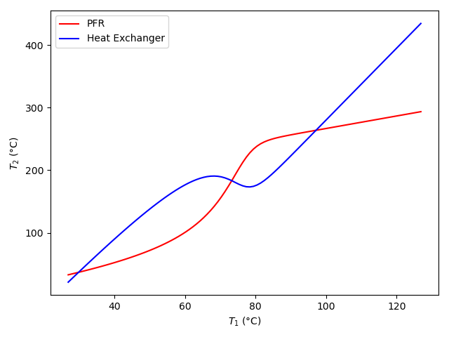
As a matter of convenience, the steady state with the lowest value of \(T_1\) will be referred to as the lower steady state, that with the greatest value of \(T_1\) as the upper steady state, and the one with the intermediate value of \(T_1\) as the middle steady state. At any value of \(T_1\), the blue curve can be thought of as the stream 2 temperature that the heat exchanger requires in order to maintain stream 1 at \(T_1\), and the red curve can be thought of as the stream 2 temperature that the PFR is capable of producing.
With that perspective, consider a system operating at either the upper or the lower steady state. If stream 1 is perturbed to a temperature \(T_1\) that is greater than its steady state temperature, the PFR cannot produce a stream 2 temperature that is large enough for the heat exchanger to maintain the perturbed stream 1 temperature. Since the stream 2 temperature is not large enough to maintain it, the perturbed stream 1 temperature will decrease until it returns to the original steady state value. In terms of Figure 16.4, if the system is perturbed slightly to the right from the upper or lower steady state, the blue curve is above the red curve, and consequently the PFR does not produce a stream 2 temperature that is high enough for the heat exchanger to maintain the new stream 1 temperature.
Similarly, if a system is operating at either the upper or the lower steady state and the stream 1 temperature is perturbed to a temperature \(T_1\) that is less than the steady state value, then PFR will produce a stream 2 temperature greater than what the heat exchanger needs in order to maintain the new temperature. With the stream 2 temperature greater than what is needed, too much heat will be transferred to stream 1, and its temperature will increase until it returns to the original steady state.
Thus, when a system is perturbed in either direction from either the upper or lower steady state, it will return to that steady state. In other words, the upper and lower steady states are stable. By the same reasoning, the middle steady state is unstable. If a system is operating at the middle steady state and the stream 1 temperature is increased slightly, the PFR will produce a stream 2 temperature in excess of what is needed to maintain the new temperature. As a consequence, the temperature of stream 1 will increase, moving it farther from the orginal middle steady state. This will continue until the system reaches the upper steady state. Similarly, if a system is operating at the middle steady state and the stream 1 temperature is decreased slightly, the PFR will produce a stream 2 temperature smaller than what is needed to maintain the new temperature. As a consequence, the temperature of stream 1 will decrease, moving it farther from the orginal middle steady state. This will continue until the system reaches the lower steady state.
16.4 Symbols used in Chapter 16
| Symbol | Meaning |
|---|---|
| \(f_i\) | Fractional conversion of reactant \(i\). |
| \(k_j\) | Rate coefficient for reaction \(j\). |
| \(k_{0,j}\) | Arrhenius pre-exponential factor for rate coefficient \(k_j\). |
| \(\dot{n}_I\) | Molar flow rate of reagent \(i\); an additional subscript denotes the flow stream. |
| \(r_j\) | Rate of reaction \(j\). |
| \(y_i\) | Gas phase mole fraction of reagent \(i\). |
| ! \(z\) | Distance from the inlet of a PFR in the axial direction. |
| \(A\) | Heat transfer area. |
| \(C_i\) | Concentration of reagent \(i\); an additional subscript denotes the flow stream. |
| \(\hat{C}_{p,i}\) | Molar heat capacity of reagent \(i\). |
| \(\tilde{C}_{p,}\) | Gravimetric heat capacity. |
| \(\breve{C}_{p,}\) | Volumetric heat capacity. |
| \(D\) | PFR diameter. |
| \(E_j\) | Arrhenius activation energy for rate coefficient \(k_j\). |
| \(P\) | Pressure. |
| \(P_i\) | Parial pressure of reagent \(i\). |
| \(R\) | Ideal gas constant. |
| \(T\) | Temperature; an additional subscript denotes the flow stream. |
| \(U\) | Heat transfer coefficient; an additional subscript denotes the type of temperature difference to be used with it. |
| \(V\) | Volume; an additional subscript denotes the equipment. |
| \(\dot{V}\) | Volumetric flow rate; an additional subscript denotes the flow stream. |
| \(\epsilon\) | Residual; an additional subscript is used to differentiate between multiple residuals. |
| \(\nu_{i,j}\) | Stoichiometric coefficient of reagent \(i\) in reaction \(j\). |
| \(\Delta H_j\) | Heat of reaction \(j\). |
| \(\Delta T\) | Temperature difference in a heat exchanger; an additional denotes the type (e. g. arithmetic mean, log-mean, or cold). |