Appendix H — Ideal Reactor Models

In this appendix, mole and energy balances are derived for each of the four kinds of ideal reactors considered in Reaction Engineering Basics.

H.1 BSTR Mole and Energy Balances

The BSTR model makes the following assumptions.

The fluid within the system is perfectly mixed.
Mass neither enters nor leaves the system while the reactions are taking place.

During the derivation of the forms of the BSTR mole and energy balances used in Reaction Engineering Basics, the following additional assumptions are made.

Kinetic energy terms and gravitational potential energy terms are negligible.
Pressure variation associated with the hydrostatic head can be ignored.
Reaction rates are normalized per fluid volume.
Exchange of energy with the surroundings takes the form of heat or mechanical work associated with shafts, moving boundaries, etc.
The fluid mixture is ideal.
- Both \(\Delta H\) and \(\Delta V\) of mixing are zero.
No phase changes occur within the system while the reactions are taking place.

H.1.1 The BSTR Mole Balance

The system being modeled is the volume of the fluid within the reactor at any instant in time. The derivation of the BSTR mole balance begins with a general balance equation written for the moles of any one species, \(i\), present in that system.

\[\text{Input Rate} + \text{Generation Rate} = \text{Output Rate} + \text{Accumulation Rate}\]

In a BSTR no mass enters or leaves the reactor while the reaction is occurring, so the Input Rate and Output Rate terms are equal to zero.

\[\text{Input Rate} = \text{Output Rate} = 0\]

With the assumption that the rate of reaction is normalized per unit volume of the reacting fluid, the rate of generation of any reagent, \(i\), due to the occurrence of reaction, \(j\), is equal to \(\nu _{i,j}V r_j\). Summing the rate of generation of \(i\) over all reactions taking place then gives Generation Rate term.

\[\text{Generation Rate} = V \sum_j \nu_{i,j}r_j\]

The instantaneous Accumulation Rate of \(i\) is simply the derrivative on \(n_i\) with respect to \(t\).

\[\text{Accumulation Rate} = \frac{dn_i}{dt}\]

Substituting into the general balance equation and rearranging yields the BSTR mole balance.

\[ \frac{dn_i}{dt} = V \sum_j \nu_{i,j}r_j \]

H.1.2 The BSTR Energy Balance

The derivation of the BSTR energy balance begins with a general balance equation, written for energy at any one instant of time during the operation of the reactor.

\[\text{Input Rate} + \text{Generation Rate} = \text{Output Rate} + \text{Accumulation Rate}\]

While no mass enters or leaves a BSTR while the reaction is occurring, it is possible for energy to enter or leave it. Here any energy that enters or leaves the system is assumed to do so either as heat or as mechanical work. The variable, \(\dot Q\), is used to represent the instantaneous net rate of heat input to the reactor from the surroundings. If heat actually leaves the reactor, \(\dot Q\) will be negative.

\[\text{Input Rate} = \dot Q\]

The variable, \(\dot W\), is used to represent the instantaneous net rate at which the reactor performs work on the surroundings.

\[\text{Output Rate} = \dot W\]

In the absence of nuclear reactions energy cannot be generated, so the Generation Rate is equal to zero. (The heat of reaction is a result of the transformation of chemical potential energy to heat, and not energy generation.)

\[\text{Generation Rate} = 0\]

With the assumption that kinetic and potential energy terms are negligible, accumulation of energy is limited to the form of internal (chemical) energy. Letting \(\hat u_i\) represent the molar specific internal energy of reagent \(i\), the instantaneous internal energy of \(i\) is then \(n_i \hat u_i\). With the assumption that the fluid is an ideal mixture (no heat of mixing), the total instantaneous internal energy is simply the sum of the instantaneous internal energies of all reagents, \(\sum_i n_i \hat u_i\), and by definition, the instantaneous rate of accumulation of internal energy is the time derivative of instantaneous internal energy.

\[\text{Accumulation Rate} = \frac{d}{dt}\left( \sum_i n_i \hat u_i \right)\]

Substitution of these terms into the general balance equation leads to a form of the BSTR energy balance that isn’t particularly useful because it is expressed in terms of specific internal energies.

\[\dot Q = \dot W + \frac{d}{dt}\left( \sum_i n_i \hat u_i \right)\]

This equation can be rearranged and the derivative taken inside the summation.

\[\sum_i \frac{d}{dt} \left( n_i \hat u_i \right) = \dot Q - \dot W\]

The specific molar internal energy of each reagent can be expressed in terms of its specific molar enthalpy and volume.

\[\sum_i \frac{d}{dt} \left( n_i \left(\hat h_i - P \hat V_i \right) \right) = \dot Q - \dot W\]

The distributive property of multiplication then can be applied.

\[\sum_i \frac{d}{dt} \left( n_i \hat h_i - n_iP \hat V_i \right) = \dot Q - \dot W\]

The derivative of the difference is then equal to the difference of the derivatives.

\[\sum_i \left( \frac{d}{dt} \left( n_i \hat h_i \right) -\frac{d}{dt} \left( n_iP \hat V_i \right) \right) = \dot Q - \dot W\]

The summation can be separated into two sums.

\[\sum_i \frac{d}{dt} \left( n_i \hat h_i \right) - \sum_i \frac{d}{dt} \left( n_iP \hat V_i \right) = \dot Q - \dot W\]

The chain rule for differentiation can be applied to both the first and second terms.

\[ \sum_i n_i \frac{d\hat h_i}{dt} + \sum_i \hat h_i \frac{dn_i}{dt} - \frac{dP}{dt} \sum_i \left( n_i \hat V_i \right) - P \sum_i \frac{d}{dt}\left( n_i \hat V_i \right) = \dot Q - \dot W\]

With the assumption that the fluid is an ideal mixture (no volume change upon mixing), \(\sum_i \left( n_i \hat V_i \right) = V\) in the third term.

\[ \sum_i n_i \frac{d\hat h_i}{dt} + \sum_i \hat h_i \frac{dn_i}{dt} - V\frac{dP}{dt} - P \sum_i \frac{d}{dt}\left( n_i \hat V_i \right) = \dot Q - \dot W\]

In the fourth term, the sum of the derivatives can be replaced with the derivative of the sum.

\[ \sum_i n_i \frac{d\hat h_i}{dt} + \sum_i \hat h_i \frac{dn_i}{dt} - V\frac{dP}{dt} - P \frac{d}{dt}\sum_i\left( n_i \hat V_i \right) = \dot Q - \dot W\]

Then in the fourth term, as before, \(\sum_i \left( n_i \hat V_i \right) = V\), because the mixture has been assumed to be ideal.

\[ \sum_i n_i \frac{d\hat h_i}{dt} + \sum_i \hat h_i \frac{dn_i}{dt} - V\frac{dP}{dt} - P \frac{dV}{dt} = \dot Q - \dot W\]

With the assumption that no phase changes occur while the reaction is taking place, the change in specific enthalpy involves only sensible heat, \(d\hat h_i = \hat C_{p,i}dT\).

\[ \left(\sum_i n_i \hat C_{p,i} \right) \frac{dT}{dt} + \sum_i \hat h_i \frac{dn_i}{dt} - V\frac{dP}{dt} - P \frac{dV}{dt} = \dot Q - \dot W\]

The BSTR mole balance can be used to express derivative of the moles of \(i\) in terms of the reaction rates.

\[ \left(\sum_i n_i \hat C_{p,i} \right) \frac{dT}{dt} + \sum_i \hat h_i V \sum_j \nu_{i,j}r_j - V\frac{dP}{dt} - P \frac{dV}{dt} = \dot Q - \dot W\]

In the second term, the distributive property of multiplication can be applied and the volume can be factored out of the summation.

\[ \left(\sum_i n_i \hat C_{p,i} \right) \frac{dT}{dt} + V\sum_i \sum_j \nu_{i,j}\hat h_i r_j - V\frac{dP}{dt} - P \frac{dV}{dt} = \dot Q - \dot W\]

In the second term, the order of the summations can be switched and the rate can be factored out of the inner sum.

\[ \left(\sum_i n_i \hat C_{p,i} \right) \frac{dT}{dt} + V \sum_j r_j \sum_i \nu_{i,j}\hat h_i - V\frac{dP}{dt} - P \frac{dV}{dt} = \dot Q - \dot W\]

With the assumption of an ideal mixture (no heat of mixing), the inner sum in the second term is equal to the standard heat of reaction, \(\sum_i \nu_{i,j}\hat h_i = \Delta H_j\).

\[ \left(\sum_i n_i \hat C_{p,i} \right) \frac{dT}{dt} + V \sum_j \left(r_j \Delta H_j \right) - V\frac{dP}{dt} - P \frac{dV}{dt} = \dot Q - \dot W\]

Rearranging to put all of the derivatives on one side of the equation leads to a more useful form of the BSTR energy balance where the temperature, pressure and volume are used instead of specific internal energies.

\[ \left(\sum_i n_i \hat C_{p,i} \right) \frac{dT}{dt} - V\frac{dP}{dt} - P \frac{dV}{dt} = \dot Q - \dot W - V \sum_j \left(r_j \Delta H_j \right) \]

H.2 SBSTR Mole and Energy Balances

In Reaction Engineering Basics, only one type of semi-batch reactor operation is considered. It is sometimes referred to as “fed-batch” operation. In this type of semi-batch processing, one or more reagents are added to the system while the reaction is taking place, but no reagents are removed from the reactor while it is operating. The SBSTR model makes the following assumptions.

The fluid within the system is perfectly mixed.
One or more reagents enter the system, but no mass leaves it while the reactor is operating.

During the derivation of the forms of the SBSTR mole and energy balances used in Reaction Engineering Basics, the following additional assumptions are made.

Kinetic energy terms and gravitational potential energy terms are negligible.
Pressure variation associated with the hydrostatic head can be ignored.
Reaction rates are normalized per fluid volume.
Exchange of energy with the surroundings takes the form of heat or mechanical work associated with shafts, moving boundaries, etc.
The fluid mixture is ideal.
- Both \(\Delta H\) and \(\Delta V\) of mixing are zero.
No phase changes occur within the system nor upon entering it while the reactor is operating.

H.2.1 The SBSTR Mole Balance

The system being modeled is the volume of the fluid within the reactor at any instant in time. The derivation of the SBSTR mole balance begins with a general balance equation, written for the moles of any one species at any one instant in time during the operation of the reactor.

\[\text{Input Rate} + \text{Generation Rate} = \text{Output Rate} + \text{Accumulation Rate}\]

The mole balance for an SBSTR is very similar to the mole balance derived above for a BSTR. The Output Rate, Generation Rate and Accumulation Rate terms are the same as for a BSTR.

\[\text{Output Rate} = 0\]

\[\text{Generation Rate} = V \sum_j \nu_{i,j}r_j\]

\[\text{Accumulation Rate} = \frac{dn_i}{dt}\]

In contrast to a BSTR, the Input Rate term does not equal zero, it is equal to the molar flow of reagent \(i\) into the system.

\[\text{Input Rate} = \dot n_{i,in}\]

Substitution into the general balance equation yields the SBSTR mole balance.

\[ \frac{dn_i}{dt} = \dot n_{i,in} + V \sum_j \nu_{i,j}r_j\]

H.2.2 The SBSTR Energy Balance

To begin, a general balance equation, written for energy at any one instant of time during the operation of the reactor is used.

\[\text{Input Rate} + \text{Generation Rate} = \text{Output Rate} + \text{Accumulation Rate}\]

The Generation Rate, Output Rate and Accumulation Rate are the same as the BSTR.

\[\text{Generation Rate} = 0\]

\[\text{Output Rate} = \dot W\]

\[\text{Accumulation Rate} = \frac{d}{dt}\left( \sum_i n_i \hat u_i \right)\]

With the assumption of negligible kinetic energy and gravitational potential energy terms, there are two input rate terms in addition to the heat entering the system, \(\dot Q\). First, the fluid must do \(PV\) or flow work on the system to enter it, and second, the reagents entering the system carry their internal energy with them.

\[\text{Input Rate} = \dot Q + P\dot V_{in} + \sum_i \dot n_{i,in}\hat u_{i,in}\]

Substitution in the general balance equation yields the SBSTR energy balance, but once again it is expressed in terms of specific internal energies, which isn’t particularly useful.

\[\dot Q + P\dot V_{in} + \sum_i \dot n_{i,in}\hat u_{i,in} = \dot W + \frac{d}{dt}\left( \sum_i n_i \hat u_i \right)\]

With the assumption that the fluid is an ideal mixture (no \(\Delta V\) of mixing), the inlet volumetric flow rate in the second term can be expressed in terms of the inlet molar flow rates and molar specific volumes, \(\dot V_{in} = \sum_i \dot n_{i,in} \hat V_{i,in}\).

\[\dot Q + P\sum_i \dot n_{i,in} \hat V_{i,in} + \sum_i \dot n_{i,in}\hat u_{i,in} = \dot W + \frac{d}{dt}\left( \sum_i n_i \hat u_i \right)\]

The second and third terms then can be combined.

\[\dot Q + \sum_i \dot n_{i,in} \left( \hat u_{i,in} + P\hat V_{i,in} \right) = \dot W + \frac{d}{dt}\left( \sum_i n_i \hat u_i \right)\]

The molar specific energies can be expressed in terms of the molar specific enthalpies and volumes, \(\hat u_{i,in} + P\hat V_{i,in} = \hat h_{i,in}\) and \(\hat u_i = \hat h_i - P\hat V_i\).

\[\dot Q + \sum_i \dot n_{i,in} \hat h_{i,in} = \dot W + \frac{d}{dt}\left( \sum_i n_i \left( \hat h_i - P\hat V_i \right) \right)\]

The distributive property of multiplication can be applied to the final term.

\[\dot Q + \sum_i \dot n_{i,in} \hat h_{i,in} = \dot W + \frac{d}{dt} \sum_i \left( n_i \hat h_i - Pn_i\hat V_i \right)\]

The final term can then be split into two summations.

\[\dot Q + \sum_i \dot n_{i,in} \hat h_{i,in} = \dot W + \frac{d}{dt} \sum_i \left( n_i \hat h_i \right) - \frac{d}{dt} \sum_i \left(Pn_i\hat V_i \right)\]

The pressure can be factored out of the final sum.

\[\dot Q + \sum_i \dot n_{i,in} \hat h_{i,in} = \dot W + \frac{d}{dt} \sum_i \left( n_i \hat h_i \right) - \frac{d}{dt} \left( P\sum_i \left(n_i\hat V_i \right) \right)\]

With the assumption that the fluid mixture is ideal, \(\sum_i \left(n_i\hat V_i \right) = V\).

\[\dot Q + \sum_i \dot n_{i,in} \hat h_{i,in} = \dot W + \frac{d}{dt} \sum_i \left( n_i \hat h_i \right) - \frac{d}{dt} \left( PV\right)\]

The derivative in the fourth term can be moved inside the summation and chain rule for differentiation then can be applied to it and the final term.

\[ \dot Q + \sum_i \dot n_{i,in} \hat h_{i,in} = \dot W + \sum_i \left( n_i \frac{d \hat h_i}{dt} + \hat h_i \frac{dn_i}{dt} \right) -V\frac{dP}{dt} - P\frac{dV}{dt} \]

The summation in the fourth term can be written as two terms.

\[ \dot Q + \sum_i \dot n_{i,in} \hat h_{i,in} = \dot W + \sum_i \left( n_i \frac{d \hat h_i}{dt}\right) + \sum_i \left( \hat h_i \frac{dn_i}{dt} \right) -V\frac{dP}{dt} - P\frac{dV}{dt} \]

With the assumption that no phase changes occur, the change in specific enthalpy in the fourth term involves only sensible heat, \(d\hat h_i = \hat C_{p,i}dT\).

\[ \dot Q + \sum_i \dot n_{i,in} \hat h_{i,in} = \dot W + \sum_i \left( n_i \hat C_{p,i}\right) \frac{dT}{dt} + \left(\sum_i \hat h_i \frac{dn_i}{dt} \right) -V\frac{dP}{dt} - P\frac{dV}{dt} \]

The time derivative of \(n_i\) can be replaced using the STSTR mole balance.

\[ \begin{split} \dot Q + \sum_i \dot n_{i,in} \hat h_{i,in} &= \dot W + \sum_i \left( n_i \hat C_{p,i}\right) \frac{dT}{dt} + \left(\sum_i \hat h_i \left(\dot n_{i,in} + V \sum_j \nu_{i,j}r_j \right)\right) \\& -V\frac{dP}{dt} - P\frac{dV}{dt} \end{split} \]

The distributive property of multiplication can be applied to the fifth term after which it can be written as two terms.

\[ \begin{split} \dot Q + \sum_i \dot n_{i,in} \hat h_{i,in} &= \dot W + \sum_i \left( n_i \hat C_{p,i}\right) \frac{dT}{dt} + \sum_i \dot n_{i,in}\hat h_i + \sum_i \left(V\hat h_i \sum_j \nu_{i,j}r_j \right) \\& -V\frac{dP}{dt} - P\frac{dV}{dt} \end{split} \]

The order of the sums in the sixth term can be switched.

\[ \begin{split} \dot Q + \sum_i \dot n_{i,in} \hat h_{i,in} &= \dot W + \sum_i \left( n_i \hat C_{p,i}\right) \frac{dT}{dt} + \sum_i \dot n_{i,in}\hat h_i + V\sum_j \sum_i \hat h_i\nu_{i,j}r_j \\& -V\frac{dP}{dt} - P\frac{dV}{dt} \end{split} \]

The rate can be factored out of the inner sum in the sixth term.

\[ \begin{split} \dot Q + \sum_i \dot n_{i,in} \hat h_{i,in} &= \dot W + \sum_i \left( n_i \hat C_{p,i}\right) \frac{dT}{dt} + \sum_i \dot n_{i,in}\hat h_i + V\sum_j r_j \sum_i \hat h_i\nu_{i,j} \\& -V\frac{dP}{dt} - P\frac{dV}{dt} \end{split} \]

With the assumption that the fluid is an ideal mixture (no \(\Delta H\) of mixing), the inner sum in the sixth term is equal to the standard heat of reaction, \(\sum_i \hat h_i\nu_{i,j} = \Delta H_j\).

\[ \begin{split} \dot Q + \sum_i \dot n_{i,in} \hat h_{i,in} &= \dot W + \sum_i \left( n_i \hat C_{p,i}\right) \frac{dT}{dt} + \sum_i \dot n_{i,in}\hat h_i + V\sum_j r_j \Delta H_j \\& -V\frac{dP}{dt} - P\frac{dV}{dt} \end{split} \]

The derivatives can all be moved to one side of the equation.

\[ \begin{split} \sum_i \left( n_i \hat C_{p,i}\right) \frac{dT}{dt} - V\frac{dP}{dt} - P\frac{dV}{dt} &= \dot Q - \dot W + \sum_i \dot n_{i,in} \hat h_{i,in} - \sum_i \dot n_{i,in}\hat h_i \\&- V\sum_j r_j \Delta H_j \end{split} \]

The third and fourth terms following the equals sign can be combined and the molar flow rate of \(i\) factored out.

\[ \sum_i \left( n_i \hat C_{p,i}\right) \frac{dT}{dt} -V\frac{dP}{dt} - P\frac{dV}{dt} = \dot Q - \dot W + \sum_i \dot n_{i,in} \left(\hat h_{i,in} - \hat h_i \right)- V\sum_j r_j \Delta H_j \]

With the assumption that no phase change occurs upon entering the system, the enthalpy difference in the third term following the equals sign involves only sensible heat and can be expressed in terms of the molar heat capacities. Doing so results in the desired form of the SBSTR energy balance, expressed in terms of temperature, pressure and volume instead of specific internal energies or enthalpies.

\[ \sum_i \left( n_i \hat C_{p,i}\right) \frac{dT}{dt} -V\frac{dP}{dt} - P\frac{dV}{dt} = \dot Q - \dot W - \sum_i \dot n_{i,in} \int_{T_{in}}^T \hat C_{p,i}dT - V\sum_j r_j \Delta H_j \]

H.3 CSTR Mole and Energy Balances

CSTRs are another variant on a perfectly-mixed reactor. They differ from BSTRs and SBSTRs in that fluid flows into and out of CSTRs. The CSTR model makes the following assumptions.

The fluid within the system is perfectly mixed.
Reagents continuously flow into and out of the system as it operates.

During the derivation of the forms of the CSTR mole and energy balances used in Reaction Engineering Basics, the following additional assumptions are made.

Kinetic energy terms and gravitational potential energy terms are negligible.
Pressure variation associated with the hydrostatic head can be ignored.
Reaction rates are normalized per fluid volume.
Exchange of energy with the surroundings takes the form of heat or mechanical work associated with shafts, moving boundaries, etc.
The fluid mixture is ideal.
- Both \(\Delta H\) and \(\Delta V\) of mixing are zero.
No phase changes occur within the system while the reactions are taking place nor upon entering the system.

H.3.1 The CSTR Mole Balance

The system being modeled is the volume of the fluid within the reactor at any instant in time. The derivation of the CSTR mole balance begins with a general balance equation written for the moles of any one species, \(i\), present in that system.

\[\text{Input Rate} + \text{Generation Rate} = \text{Output Rate} + \text{Accumulation Rate}\]

The Input Rate and Output Rate terms are straightforward.

\[\text{Input Rate} = \dot n_{i,in}\]

\[\text{Output Rate} = \dot n_i\]

The Generation Rate is the same as the BSTR and SBSTR.

\[\text{Generation Rate} = V \sum_j \nu_{i,j}r_j\]

The Accumulation Rate term is also the same as the BSTR and SBSTR, but the equation will be easier to work with if the accumulation is expressed in terms of the molar flow rate of \(i\), \(\dot n_i\), instead of the number of moles of \(i\), \(n_i\). This can be accomplished by noting that the number of moles is equal to the product of the volume and the concentration, \(n_i = C_iV\). With the assumption that the reactor is perfectly mixed, the concentration within the reactor is equal to the concentration leaving the reactor, \(C_i = \frac{\dot n_i}{\dot V}\).

\[\text{Accumulation Rate} = \frac{dn_i}{dt} = \frac{d}{dt}\left( \frac{\dot n_iV}{\dot V} \right)\]

Substitution into the general balance equation yields the CSTR mole balance equation.

\[\dot n_{i,in} + V \sum_j \nu_{i,j}r_j = \dot n_i + \frac{d}{dt}\left( \frac{\dot n_iV}{\dot V} \right)\]

This equation can be rearranged to put the derivative on one side of the equation and the remaining terms on the other.

\[\frac{d}{dt}\left( \frac{\dot n_iV}{\dot V} \right) = \dot n_{i,in} - \dot n_i + V \sum_j \nu_{i,j}r_j\]

Applying the chain rule for differentiation then yields the desired form of the CSTR mole balance equation.

\[\frac{V}{\dot V}\frac{d \dot n_i}{dt} + \frac{\dot n_i}{\dot V}\frac{dV}{dt} - \frac{\dot n_iV}{\dot V^2}\frac{d \dot V}{dt} = \dot n_{i,in} - \dot n_i + V \sum_j \nu_{i,j}r_j\]

H.3.2 The CSTR Energy Balance

The CSTR energy balance begins with a general balance equation written for energy at any one instant of time during the operation of the reactor.

\[\text{Input Rate} + \text{Generation Rate} = \text{Output Rate} + \text{Accumulation Rate}\]

The Input Rate and Generation Rate are the same as the SBSTR.

\[\text{Input Rate} = \dot Q + P\dot V_{in} + \sum_i \dot n_{i,in}\hat u_{i,in}\]

\[\text{Generation Rate} = 0\]

The Output Rate includes the shaft work term that appears in the BSTR and SBSTR and adds flow work and internal energy of the fluid leaving the reactor that are analogous to the input terms.

\[\text{Output Rate} = \dot W + P\dot V + \sum_i \dot n_i\hat u_i\]

The Accumulation Rate term is the same as a BSTR or SBSTR, but as it was in the CSTR mole balance, it is convient to express it in terms of the molar flow rate, \(\dot n_i\), instead of the moles, \(n_i\). This is accomplished in the same way as in the CSTR mole balance.

\[\text{Accumulation Rate} = \frac{d}{dt}\left( \sum_i n_i \hat u_i \right) = \frac{d}{dt}\left( \sum_i \frac{\dot n_i \hat u_iV}{\dot V} \right)\]

Substituting into the general balance equation yields a form of the CSTR energy balance expressed in terms of specific internal energies.

\[\dot Q + P\dot V_{in} + \sum_i \dot n_{i,in}\hat u_{i,in} = \dot W + P\dot V + \sum_i \dot n_i\hat u_i + \frac{d}{dt}\left( \sum_i \frac{\dot n_i \hat u_iV}{\dot V} \right)\]

With the assumption that the fluid is an ideal mixture, no \(\Delta V\) of mixing, the volumetric flow rates in the second and fifth terms are equal to the sums of the molar flow rates times the molar specific volumes.

\[ \begin{split}\dot Q + P\sum_i\left( \dot n_{i,in}\hat V_{i,in} \right) + \sum_i \dot n_{i,in}\hat u_{i,in} &= \dot W + P\sum_i\left( \dot n_i\hat V_i \right) + \sum_i \dot n_i\hat u_i \\&+ \frac{d}{dt}\left( \sum_i \frac{\dot n_i \hat u_iV}{\dot V} \right) \end{split} \]

The second and third summations and the fifth and sixth summations can each be combined.

\[\dot Q + \sum_i\left(\dot n_{i,in}\left( P \hat V_{i,in} + \hat u_{i,in} \right)\right) = \dot W + \sum_i\left( \dot n_i\left(P\hat V_i + \hat u_i \right) \right) + \frac{d}{dt}\left( \sum_i \frac{\dot n_i \hat u_iV}{\dot V} \right)\]

The specific energy can be expressed in terms of the specific enthalpy and specific volume, \(\hat u_{i,in} + P\hat V_{i,in} = \hat h_{i,in}\) and \(\hat u_i + P\hat V_i = \hat h_i\).

\[\dot Q + \sum_i\dot n_{i,in} \hat h_{i,in} = \dot W + \sum_i \dot n_i \hat h_i + \frac{d}{dt}\left( \sum_i \frac{\dot n_i \hat u_iV}{\dot V} \right)\]

Similarly, the specific internal energy in the last term can be expressed in terms of the specific enthalpy and volume.

\[\dot Q + \sum_i\dot n_{i,in} \hat h_{i,in} = \dot W + \sum_i \dot n_i \hat h_i + \frac{d}{dt}\left( \sum_i \left( \hat h_i - P\hat V_i \right)\frac{\dot n_i V}{\dot V} \right)\]

The distributive property of multiplication can be applied to the last term.

\[\dot Q + \sum_i\dot n_{i,in} \hat h_{i,in} = \dot W + \sum_i \dot n_i \hat h_i + \frac{d}{dt} \sum_i \left( \frac{\dot n_i\hat h_i V}{\dot V} - \frac{\dot n_i VP\hat V_i}{\dot V} \right)\]

The last term can be split into two terms.

\[\dot Q + \sum_i\dot n_{i,in} \hat h_{i,in} = \dot W + \sum_i \dot n_i \hat h_i + \frac{d}{dt} \sum_i \left( \frac{\dot n_i\hat h_i V}{\dot V} \right) - \frac{d}{dt} \sum_i \left( \frac{\dot n_i VP\hat V_i}{\dot V} \right)\]

Then \(\frac{PV}{\dot V}\) can be factored out of the final summation.

\[\dot Q + \sum_i\dot n_{i,in} \hat h_{i,in} = \dot W + \sum_i \dot n_i \hat h_i + \frac{d}{dt} \sum_i \left( \frac{\dot n_i\hat h_i V}{\dot V} \right) - \frac{d}{dt} \left(\frac{PV}{\dot V} \sum_i \left(\dot n_i \hat V_i \right)\right)\]

With the assumption that the mixture is ideal \(\left(\sum_i \left(\dot n_i \hat V_i \right) = \dot V\right)\), the final term can be simplified.

\[\dot Q + \sum_i\dot n_{i,in} \hat h_{i,in} = \dot W + \sum_i \dot n_i \hat h_i + \frac{d}{dt} \sum_i \left( \frac{\dot n_i\hat h_i V}{\dot V} \right) - \frac{d}{dt} \left( PV\right)\]

The chain rule can be applied to the fifth term.

\[ \begin{split} \dot Q + \sum_i\dot n_{i,in} \hat h_{i,in} &= \dot W + \sum_i \dot n_i \hat h_i \\&+ \sum_i \hat h_i\frac{d}{dt}\left( \frac{\dot n_i V}{\dot V} \right) + \sum_i \left( \frac{\dot n_i V}{\dot V} \right)\frac{d\hat h_i}{dt} - \frac{d}{dt} \left( PV\right) \end{split} \]

With the assumption of no phase changes, changes in enthalpy only involve sensible heat and the time-derivative of the specific enthalpy can be expressed in terms of the heat capacity and the temperature.

\[ \begin{split} \dot Q + \sum_i\dot n_{i,in} \hat h_{i,in} &= \dot W + \sum_i \dot n_i \hat h_i \\&+ \sum_i \hat h_i\left[\frac{d}{dt}\left( \frac{\dot n_i V}{\dot V} \right)\right] + \sum_i \left( \frac{\dot n_i \hat C_{p,i} V}{\dot V} \right)\frac{dT}{dt} - \frac{d}{dt} \left( PV\right) \end{split} \]

The term containing square brackets can be moved to the end of the equation.

\[ \begin{split} \dot Q + \sum_i\dot n_{i,in} \hat h_{i,in} &= \dot W + \sum_i \dot n_i \hat h_i + \sum_i \left( \frac{\dot n_i \hat C_{p,i} V}{\dot V} \right)\frac{dT}{dt} - \frac{d}{dt} \left( PV\right) \\&+ \sum_i \hat h_i\left[\frac{d}{dt}\left( \frac{\dot n_i V}{\dot V} \right)\right] \end{split} \]

The chain rule can be applied to the term containing square brackets.

\[ \begin{split} \dot Q + \sum_i\dot n_{i,in} \hat h_{i,in} &= \dot W + \sum_i \dot n_i \hat h_i + \sum_i \left( \frac{\dot n_i \hat C_{p,i} V}{\dot V} \right)\frac{dT}{dt} - \frac{d}{dt} \left( PV\right) \\&+ \sum_i \hat h_i\left[\frac{V}{\dot V}\frac{d \dot n_i}{dt} + \frac{\dot n_i}{\dot V}\frac{dV}{dt} - \frac{\dot n_iV}{\dot V^2}\frac{d \dot V}{dt}\right] \end{split} \]

The term in the square brackets is equal to one side of the CSTR mole balance. The other side of the CSTR mole balance can be substituted in its place.

\[ \begin{split} \dot Q + \sum_i\dot n_{i,in} \hat h_{i,in} &= \dot W + \sum_i \dot n_i \hat h_i + \sum_i \left( \frac{\dot n_i \hat C_{p,i} V}{\dot V} \right)\frac{dT}{dt} - \frac{d}{dt} \left( PV\right) \\&+ \sum_i \hat h_i\left[\dot n_{i,in} - \dot n_i + V \sum_j \nu_{i,j}r_j\right] \end{split} \]

The distributive property of multiplication can be applied to the term with the square brackets.

\[ \begin{split} \dot Q + \sum_i\dot n_{i,in} \hat h_{i,in} &= \dot W + \sum_i \dot n_i \hat h_i + \sum_i \left( \frac{\dot n_i \hat C_{p,i} V}{\dot V} \right)\frac{dT}{dt} - \frac{d}{dt} \left( PV\right) \\&+ \sum_i \hat h_i\dot n_{i,in} - \sum_i \hat h_i\dot n_i + V\sum_i \hat h_i \sum_j \nu_{i,j}r_j \end{split} \]

The first term on the second line can be moved to the other side of the equation, and two other terms cancel out.

\[ \begin{split} \dot Q + \sum_i\dot n_{i,in} \hat h_{i,in} - \sum_i \hat h_i\dot n_{i,in} &= \dot W + \cancel{\sum_i \dot n_i \hat h_i} + \sum_i \left( \frac{\dot n_i \hat C_{p,i} V}{\dot V} \right)\frac{dT}{dt} \\&- \frac{d}{dt} \left( PV\right) - \cancel{\sum_i \hat h_i\dot n_i} + \sum_i \hat h_iV \sum_j \nu_{i,j}r_j \end{split} \]

The second and third terms can be combined.

\[ \begin{split} \dot Q + \sum_i\dot n_{i,in} \left( \hat h_{i,in} - \hat h_i \right) &= \dot W + \sum_i \left( \frac{\dot n_i \hat C_{p,i} V}{\dot V} \right)\frac{dT}{dt} - \frac{d}{dt} \left( PV\right) \\&+ V\sum_i \hat h_i \sum_j \nu_{i,j}r_j \end{split} \]

The distributive property of multiplication can be applied to the last term.

The order of the sums in the last term can be switched and \(r_j\) can be factored out of the inner summation.

With the assumption of no phase changes, the specific enthalpy difference in the second term can be expressed in terms of the heat capacity and temperature, and with the assumption that the fluid is an ideal mixture (no \(\Delta H\) of mixing), the final summation is simply equal to the heat of reaction \(j\).

\[\dot Q - \sum_i\dot n_{i,in} \int_{T_{in}}^T \hat C_{p,i}dT = \dot W + \sum_i \left( \frac{\dot n_i \hat C_{p,i} V}{\dot V} \right)\frac{dT}{dt} - \frac{d}{dt} \left( PV\right) + V\sum_j r_j \Delta H_j\]

The derivatives can be moved to one side of the equation.

\[\sum_i \left( \frac{\dot n_i \hat C_{p,i} V}{\dot V} \right)\frac{dT}{dt} - \frac{d}{dt} \left( PV\right) = \dot Q - \dot W - \sum_i\dot n_{i,in} \int_{T_{in}}^T \hat C_{p,i}dT - V\sum_j r_j \Delta H_j\]

Finally, \(V\) and \(\dot V\) can be factored out of the first term and the chain rule can be applied to the second term, yielding the desired form of the CSTR energy balance.

\[ \begin{split} \frac{V}{\dot V}\sum_i \left( \dot n_i \hat C_{p,i} \right)\frac{dT}{dt} - P\frac{dV}{dt} - V \frac{dP}{dt} &= \dot Q - \dot W - \sum_i\dot n_{i,in} \int_{T_{in}}^T \hat C_{p,i}dT \\&- V\sum_j r_j \Delta H_j \end{split} \]

H.4 PFR Mole and Energy Balances

The PFR model makes the following assumptions.

The reactor is a cylinder with fluid continuously flowing in one end and out the other.
The fluid velocity does not vary across the diameter of the reactor; i. e. there is plug flow.
- Heat and mass are perfectly mixed across the radius.
- Heat and mass do not mix at all along the axis.
If there is a packed bed of catalyst particles within the reactor it is assumed that
- there are no concentration gradients and no temperature gradients within the fluid near the external surfaces of the catalyst particles,
- there are no concentration gradients and no temperature gradients within the fluid that is in the pores inside the catalyst particles, and consequently,
- the reactor volume can be treated as a single phase (the so-called pseudo homogeneous model) by properly re-normalizing the rate of reaction.

During the derivation of the forms of the PFR mole and energy balances used in Reaction Engineering Basics, the following additional assumptions are made.

The reactor diameter is constant.
Kinetic energy terms and gravitational potential energy terms are negligible.
Reaction rates are normalized per fluid volume.
Exchange of energy with the surroundings takes the form of heat that is transferred through the wall of the reactor.
Mechanical work is not performed on or by the system.
The fluid mixture is ideal.
- Both \(\Delta H\) and \(\Delta V\) of mixing are zero.
No phase changes occur within or upon entering the system.

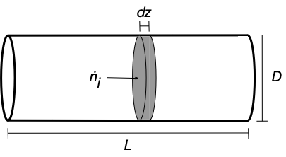
Unlike the perfectly mixed stirred tank reactors, the composition in an ideal PFR is not uniform; it changes along the length of the reactor. As a consequence, it becomes necessary to write the mole and energy balance equations on a differential element of reactor volume and then take the limit as the size of this element goes to zero. With the assumption of perfect mixing in the radial direction, in the limit where its thickness goes to zero, the volume element is perfectly mixed. Here, we will assume that the reactor is cylindrical with a constant diameter, D, and a length, L, as shown in Figure H.1 which additionally shows a differentially thick cross section that will be used in formulating the mole and energy balances.

H.4.1 The PFR Mole Balance

The system being modeled is the fluid within the differential volume element of axial thickness, \(dz\), and diameter, \(D\), at any instant in time. The derivation begins with a general balance equation written for the moles of any one species, \(i\), present in the system.

\[\text{Input Rate} + \text{Generation Rate} = \text{Output Rate} + \text{Accumulation Rate}\]

As with the CSTR, the Input Rate and Output Rate terms are simply equal to the molar flow rates at \(z\) and \(z + dz\), respectively.

\[\text{Input Rate} = \dot n_i \biggr\rvert_z\]

\[\text{Output Rate} = \dot n_i \biggr\rvert_{z+dz}\]

With the assumption that the rates are normalized per fluid volume, the rate of generation of species \(i\) via reaction \(j\) is the volume of the fluid element, \(\frac{\pi D^2}{4}dz\), times the rate of generation of \(i\) per fluid volume, \(\nu_{i,j}r_j\). The Generation Rate term then is the sum over all reactions.

\[\text{Generation Rate} = \frac{\pi D^2}{4}dz \sum_j \nu_{i,j}r_j\]

The Accumulation Rate is the instantaneous time-derivative of the number of moles in the differential element. The number of moles equals the volume of the differential element times the concentration of the species. In a flow system, the concentration is the ratio of the molar flow rate to the volumetric flow rate.

\[\text{Accumulation Rate} = \frac{\partial n_i}{\partial t} = \frac{\pi D^2}{4}dz \frac{\partial}{\partial t}\left( \frac{\dot n_i \big\rvert_z}{\dot V} \right)\]

Substitution into the general balance equation yields a mole balance expressed in terms of the differential thickness of the fluid element.

\[\dot n_i \biggr\rvert_z + \frac{\pi D^2}{4}dz \sum_j \nu_{i,j}r_j = \dot n_i \biggr\rvert_{z+dz} + \frac{\pi D^2}{4}dz \frac{\partial}{\partial t}\left( \frac{\dot n_i \big\rvert_z}{\dot V} \right)\]

That equation can be rearranged and divided by \(dz\).

\[\frac{\dot n_i \biggr\rvert_{z+dz} - \dot n_i \biggr\rvert_z}{dz}=\frac{\pi D^2}{4}\sum_j \nu_{i,j}r_j - \frac{\pi D^2}{4} \frac{\partial}{\partial t}\left( \frac{\dot n_i \big\rvert_z}{\dot V} \right)\]

Taking the limit as \(dz\) approaches zero yields the mole balance in the form of a partial differential equation.

\[\frac{\partial \dot n_i}{\partial z}=\frac{\pi D^2}{4}\sum_j \nu_{i,j}r_j - \frac{\pi D^2}{4} \frac{\partial}{\partial t}\left( \frac{\dot n_i \big\rvert_z}{\dot V} \right)\]

Applying the chain rule and moving all of the derivatives to one side of the equation leads to the desired form of the PFR mole balance.

\[\frac{\partial \dot n_i}{\partial z} + \frac{\pi D^2}{4\dot V} \frac{\partial\dot n_i}{\partial t} - \frac{\pi D^2\dot n_i}{4\dot V^2} \frac{\partial \dot V}{\partial t} =\frac{\pi D^2}{4}\sum_j \nu_{i,j}r_j \]

H.4.2 The PFR Energy Balance

The PFR energy balance begins with a general balance on the same fluid element, Figure H.1, as was used for the PFR mole balance only written for energy at any one instant of time during the operation of the reactor.

\[\text{Input Rate} + \text{Generation Rate} = \text{Output Rate} + \text{Accumulation Rate}\]

As was the case for the SBSTR and CSTR, the Input Rate term includes internal energy carried into the volume by the fluid, flow work done by the fluid on the volume element and heat transfer through the wall of the differential element. It is assumed that the heat transfer coefficient, \(U\), is constant.

\[\text{Input Rate} = \sum_i \left( \dot n_i \hat u_i \right) \biggr\rvert_z + \left( P\dot V \right)\biggr\rvert_z + \pi D U\left( T_e - T \right)dz\]

The Output Rate term is also like that for the CSTR except that there is no shaft work for a PFR.

\[\text{Output Rate} = \sum_i \left( \dot n_i \hat u_i \right) \biggr\rvert_{z+dz} + \left( P\dot V \right)\biggr\rvert_{z+dz}\]

As with all of the reactors, the Generation Rate is zero.

\[\text{Generation Rate} = 0\]

The Rate of Accumulation term is like that for the CSTR except that the volume is the volume of the differential element. Also, because there are quantities that vary with both axial position and time, the derivative is a partial derivative.

\[\text{Accumulation Rate} = \sum_i \frac{\partial}{\partial t} \left( \frac{\pi D^2}{4} \left( \frac{\dot n_i \hat u_i}{\dot V} \right)dz \right)\]

The Input Rate, Generation Rate, Output Rate and Accumulation Rate terms can be substituted into the general balance equation.

\[ \begin{split} \sum_i \left( \dot n_i \hat u_i \right) \biggr\rvert_z + \left( P\dot V \right)\biggr\rvert_z + \pi D U\left( T_e - T \right)dz &= \sum_i \left( \dot n_i \hat u_i \right) \biggr\rvert_{z+dz} + \left( P\dot V \right)\biggr\rvert_{z+dz} \\&+ \sum_i \frac{\partial}{\partial t} \left( \frac{\pi D^2}{4} \left( \frac{\dot n_i \hat u_i}{\dot V} \right)dz \right) \end{split} \]

With the assumption that the fluid is an ideal mixture with no \(\Delta V\) of mixing, the volumetric flow rates can be related to the molar flow rates and the molar specific volumes, \(\dot V = \sum_i \dot n_i \hat V_i\).

\[ \begin{split} \sum_i \left( \dot n_i \hat u_i \right) \biggr\rvert_z + \left( P \sum_i \dot n_i \hat V_i \right)\biggr\rvert_z &+ \pi D U\left( T_e - T \right)dz = \sum_i \left( \dot n_i \hat u_i \right) \biggr\rvert_{z+dz} \\&+ \left( P \sum_i \dot n_i \hat V_i \right)\biggr\rvert_{z+dz} + \sum_i \frac{\partial}{\partial t} \left( \frac{\pi D^2}{4} \left( \frac{\dot n_i \hat u_i}{\dot V} \right)dz \right) \end{split} \]

The first two terms can be combined and \(\dot n_i\) can be factored out, and the same can be done with the first two terms following the equals sign.

\[ \begin{split} \sum_i \left(\dot n_i \left( \hat u_i + P \hat V_i\right) \right) \biggr\rvert_z + \pi D U\left( T_e - T \right)dz &= \sum_i \left(\dot n_i \left( \hat u_i + P \hat V_i\right) \right) \biggr\rvert_{z+dz} \\&+ \sum_i \frac{\partial}{\partial t} \left( \frac{\pi D^2}{4} \left( \frac{\dot n_i \hat u_i}{\dot V} \right)dz \right) \end{split} \]

The specific internal energy can be expressed in terms of the specfic volume and the specific enthalpy (\(\hat u_i + P \hat V_i = \hat h_i\)).

\[\sum_i \left(\dot n_i \hat h_i \right) \biggr\rvert_z + \pi D U\left( T_e - T \right)dz = \sum_i \left(\dot n_i\hat h_i \right) \biggr\rvert_{z+dz} + \sum_i \frac{\partial}{\partial t} \left( \frac{\pi D^2}{4} \left( \frac{\dot n_i \hat u_i}{\dot V} \right)dz \right) \]

The equation can be rearranged and divided by \(dz\).

\[\sum_i \frac{\left(\dot n_i\hat h_i \right) \biggr\rvert_{z+dz}-\left(\dot n_i\hat h_i \right) \biggr\rvert_z}{dz} = \pi D U\left( T_e - T \right) - \frac{\pi D^2}{4} \sum_i \frac{\partial}{\partial t} \left( \frac{\dot n_i \hat u_i}{\dot V} \right)\]

In the limit where \(dz\) goes to zero, the left side of the equation becomes a partial derivative.

\[\sum_i \frac{\partial}{\partial z} \left( \dot n_i\hat h_i \right) = \pi D U\left( T_e - T \right) - \frac{\pi D^2}{4} \sum_i \frac{\partial}{\partial t} \left( \frac{\dot n_i \hat u_i}{\dot V} \right) \]

The chain rule can be applied to both derivatives and they can be split into separate summations.

\[ \begin{split} \sum_i \dot n_i \frac{\partial \hat h_i}{\partial z} + \sum_i \hat h_i \frac{\partial \dot n_i}{\partial z} &= \pi D U\left( T_e - T \right) - \frac{\pi D^2}{4\dot V} \sum_i \hat u_i \frac{\partial\dot n_i }{\partial t} + \frac{\pi D^2}{4\dot V^2} \sum_i \dot n_i\hat u_i \frac{\partial \dot V}{\partial t} \\&-\frac{\pi D^2}{4\dot V} \sum_i \dot n_i \frac{\partial \hat u_i}{\partial t} \end{split} \]

As before, the specific internal energy can be expressed in terms of the specific enthalpy.

\[ \begin{split} \sum_i \dot n_i \frac{\partial \hat h_i}{\partial z} + \sum_i \hat h_i \frac{\partial \dot n_i}{\partial z} &= \pi D U\left( T_e - T \right) \\&- \frac{\pi D^2}{4\dot V} \sum_i \hat h_i \frac{\partial\dot n_i }{\partial t} + \frac{\pi D^2}{4\dot V}\sum_i P\hat V_i \frac{\partial\dot n_i }{\partial t} \\&+ \frac{\pi D^2}{4\dot V^2} \sum_i \dot n_i\hat h_i \frac{\partial \dot V}{\partial t} - \frac{\pi D^2}{4\dot V^2} \sum_i \dot n_iP\hat V_i \frac{\partial \dot V}{\partial t} \\&-\frac{\pi D^2}{4\dot V} \sum_i \dot n_i \frac{\partial \hat h_i}{\partial t} + \frac{\pi D^2}{4\dot V} \sum_i \dot n_i \frac{\partial}{\partial t}\left( P\hat V_i \right) \end{split} \]

All terms including \(\hat h_i\) can be gathered.

\[ \begin{split} \sum_i \hat h_i \frac{\partial \dot n_i}{\partial z} + \frac{\pi D^2}{4\dot V} \sum_i \hat h_i \frac{\partial\dot n_i }{\partial t} - \frac{\pi D^2}{4\dot V^2} \sum_i \dot n_i\hat h_i \frac{\partial \dot V}{\partial t} &= \pi D U\left( T_e - T \right) - \sum_i \dot n_i \frac{\partial \hat h_i}{\partial z} \\ &+\frac{\pi D^2}{4\dot V} \sum_i P\hat V_i \frac{\partial\dot n_i }{\partial t} \\ &-\frac{\pi D^2}{4\dot V^2} \sum_i \dot n_iP\hat V_i \frac{\partial \dot V}{\partial t}\\ &+\frac{\pi D^2}{4\dot V} \sum_i \dot n_i \frac{\partial}{\partial t}\left( P\hat V_i \right) \\ &-\frac{\pi D^2}{4\dot V} \sum_i \dot n_i \frac{\partial \hat h_i}{\partial t} \end{split} \]

The specific enthalpy can be factored out of those terms.

\[ \begin{split} \sum_i \left(\hat h_i \left[ \frac{\partial \dot n_i}{\partial z} + \frac{\pi D^2}{4\dot V} \frac{\partial\dot n_i }{\partial t} - \frac{\pi D^2}{4\dot V^2} \dot n_i \frac{\partial \dot V}{\partial t} \right] \right) &= \pi D U\left( T_e - T \right) - \sum_i \dot n_i \frac{\partial \hat h_i}{\partial z} \\ &+\frac{\pi D^2}{4\dot V} \sum_i P\hat V_i \frac{\partial\dot n_i }{\partial t} \\ &-\frac{\pi D^2}{4\dot V^2} \sum_i \dot n_iP\hat V_i \frac{\partial \dot V}{\partial t}\\ &+\frac{\pi D^2}{4\dot V} \sum_i \dot n_i \frac{\partial}{\partial t}\left( P\hat V_i \right)\\ &-\frac{\pi D^2}{4\dot V} \sum_i \dot n_i \frac{\partial \hat h_i}{\partial t} \end{split} \]

The term in square brackets is equal to the left side of the PFR mole balance equation. It can be replaced with the right side of the PFR mole balance equation.

\[ \begin{split} \sum_i \left(\hat h_i \left[\frac{\pi D^2}{4}\sum_j \nu_{i,j}r_j \right] \right) &= \pi D U\left( T_e - T \right) - \sum_i \dot n_i \frac{\partial \hat h_i}{\partial z} \\ &+\frac{\pi D^2}{4\dot V} \sum_i P\hat V_i \frac{\partial\dot n_i }{\partial t} \\ &-\frac{\pi D^2}{4\dot V^2} \sum_i \dot n_iP\hat V_i \frac{\partial \dot V}{\partial t}\\ &+\frac{\pi D^2}{4\dot V} \sum_i \dot n_i \frac{\partial}{\partial t}\left( P\hat V_i \right)\\ &-\frac{\pi D^2}{4\dot V} \sum_i \dot n_i \frac{\partial \hat h_i}{\partial t} \end{split} \]

The distributive property of multiplication can be applied to the first term and the constant area term can be factored out.

\[ \begin{split} \frac{\pi D^2}{4}\sum_i \sum_j \hat h_i\nu_{i,j}r_j &= \pi D U\left( T_e - T \right) - \sum_i \dot n_i \frac{\partial \hat h_i}{\partial z} \\ &+ \frac{\pi D^2}{4\dot V}\sum_i P\hat V_i \frac{\partial\dot n_i }{\partial t} \\ &-\frac{\pi D^2}{4\dot V^2} \sum_i \dot n_iP\hat V_i \frac{\partial \dot V}{\partial t}\\ &+\frac{\pi D^2}{4\dot V} \sum_i \dot n_i \frac{\partial}{\partial t}\left( P\hat V_i \right)\\ &-\frac{\pi D^2}{4\dot V} \sum_i \dot n_i \frac{\partial \hat h_i}{\partial t} \end{split} \]

The order of the summations in the first term can be switched and the rate can be factored out of the inner summation.

\[ \begin{split} \frac{\pi D^2}{4}\sum_j\left( r_j\sum_i \hat h_i\nu_{i,j}\right) &= \pi D U\left( T_e - T \right) - \sum_i \dot n_i \frac{\partial \hat h_i}{\partial z} \\ &+ \frac{\pi D^2}{4\dot V}\sum_i P\hat V_i \frac{\partial\dot n_i }{\partial t} \\ &-\frac{\pi D^2}{4\dot V^2} \sum_i \dot n_iP\hat V_i \frac{\partial \dot V}{\partial t}\\ &+\frac{\pi D^2}{4\dot V} \sum_i \dot n_i \frac{\partial}{\partial t}\left( P\hat V_i \right)\\ &-\frac{\pi D^2}{4\dot V} \sum_i \dot n_i \frac{\partial \hat h_i}{\partial t} \end{split} \]

With the assumption that the fluid is an ideal mixture with no \(\Delta H\) of mixing, the second sum within the first term is simply the heat of reaction \(j\).

\[ \begin{split} \frac{\pi D^2}{4}\sum_j r_j \Delta H_j &= \pi D U\left( T_e - T \right) - \sum_i \dot n_i \frac{\partial \hat h_i}{\partial z} \\ &+\frac{\pi D^2}{4\dot V} \sum_i P\hat V_i \frac{\partial\dot n_i }{\partial t} \\ &-\frac{\pi D^2}{4\dot V^2} \sum_i \dot n_iP\hat V_i \frac{\partial \dot V}{\partial t}\\ &+\frac{\pi D^2}{4\dot V} \sum_i \dot n_i \frac{\partial}{\partial t}\left( P\hat V_i \right)\\ &-\frac{\pi D^2}{4\dot V} \sum_i \dot n_i \frac{\partial \hat h_i}{\partial t} \end{split} \]

With the assumption of no phase changes, the derivative of the specific enthalpy involves only sensible heat and can be expressed in terms of the heat capacity and temperature.

\[ \begin{split} \frac{\pi D^2}{4}\sum_j r_j \Delta H_j &= \pi D U\left( T_e - T \right) - \left(\sum_i \dot n_i \hat C_{p,i} \right) \frac{\partial T}{\partial z} \\ &+\frac{\pi D^2}{4\dot V} \sum_i P\hat V_i \frac{\partial\dot n_i }{\partial t} \\ &-\frac{\pi D^2}{4\dot V^2} \sum_i \dot n_iP\hat V_i \frac{\partial \dot V}{\partial t}\\ &+\frac{\pi D^2}{4\dot V} \sum_i \dot n_i \frac{\partial}{\partial t}\left( P\hat V_i \right)\\ &-\frac{\pi D^2}{4\dot V} \sum_i \dot n_i \frac{\partial \hat h_i}{\partial t} \end{split} \]

The chain rule can be applied to the term on the fourth line.

\[ \begin{split} \frac{\pi D^2}{4}\sum_j r_j \Delta H_j &= \pi D U\left( T_e - T \right) - \left(\sum_i \dot n_i \hat C_{p,i} \right) \frac{\partial T}{\partial z} \\ &+\frac{\pi D^2}{4\dot V} \sum_i P\hat V_i \frac{\partial\dot n_i }{\partial t} \\ &-\frac{\pi D^2}{4\dot V^2} \sum_i \dot n_iP\hat V_i \frac{\partial \dot V}{\partial t}\\ &+\frac{\pi D^2}{4\dot V} \sum_i \dot n_iP \frac{\partial \hat V_i}{\partial t}\\ &+\frac{\pi D^2}{4\dot V} \sum_i \dot n_i\hat V_i \frac{\partial P}{\partial t}\\ &-\frac{\pi D^2}{4\dot V} \sum_i \dot n_i \frac{\partial \hat h_i}{\partial t} \end{split} \]

Common quantities can be factored out of each of the sums on the second through fifth lines.

\[ \begin{split} \frac{\pi D^2}{4}\sum_j r_j \Delta H_j &= \pi D U\left( T_e - T \right) - \left(\sum_i \dot n_i \hat C_{p,i} \right) \frac{\partial T}{\partial z} \\ &+\frac{\pi D^2P}{4\dot V} \sum_i \hat V_i \frac{\partial\dot n_i }{\partial t} \\ &-\frac{\pi D^2P}{4\dot V^2} \frac{\partial \dot V}{\partial t}\sum_i \dot n_i\hat V_i \\ &+\frac{\pi D^2P}{4\dot V} \sum_i \dot n_i \frac{\partial \hat V_i}{\partial t}\\ &+\frac{\pi D^2}{4\dot V} \frac{\partial P}{\partial t}\sum_i \dot n_i\hat V_i \\ &-\frac{\pi D^2}{4\dot V} \sum_i \dot n_i \frac{\partial \hat h_i}{\partial t} \end{split} \]

As above, with the assumption that the fluid is an ideal mixture, \(\sum_i \dot n_i \hat V_i = \dot V\).

\[ \begin{split} \frac{\pi D^2}{4}\sum_j r_j \Delta H_j &= \pi D U\left( T_e - T \right) - \left(\sum_i \dot n_i \hat C_{p,i} \right) \frac{\partial T}{\partial z} \\ &+\frac{\pi D^2P}{4\dot V} \sum_i \hat V_i \frac{\partial\dot n_i }{\partial t} \\ &-\frac{\pi D^2P}{4\dot V^2} \frac{\partial \dot V}{\partial t}\dot V \\ &+\frac{\pi D^2P}{4\dot V} \sum_i \dot n_i \frac{\partial \hat V_i}{\partial t}\\ &+\frac{\pi D^2}{4\dot V} \frac{\partial P}{\partial t} \dot V \\ &-\frac{\pi D^2}{4\dot V} \sum_i \dot n_i \frac{\partial \hat h_i}{\partial t} \end{split} \]

The volumetric flow rate appears in both the numerator and denominator of the terms on the third and fifth lines and can be canceled.

\[ \begin{split} \frac{\pi D^2}{4}\sum_j r_j \Delta H_j &= \pi D U\left( T_e - T \right) - \left(\sum_i \dot n_i \hat C_{p,i} \right) \frac{\partial T}{\partial z} \\ &+\frac{\pi D^2P}{4\dot V} \sum_i \hat V_i \frac{\partial\dot n_i }{\partial t} \\ &-\frac{\pi D^2P}{4\dot V} \frac{\partial \dot V}{\partial t} \\ &+\frac{\pi D^2P}{4\dot V} \sum_i \dot n_i \frac{\partial \hat V_i}{\partial t}\\ &+\frac{\pi D^2}{4} \frac{\partial P}{\partial t} \\ &-\frac{\pi D^2}{4\dot V} \sum_i \dot n_i \frac{\partial \hat h_i}{\partial t} \end{split} \]

With the assumption that the fluids is an ideal mxiture, the derivative of the volumetric flow rate in the term on the third line can be expressed in terms of the molar flow rates and specific volumes.

\[ \begin{split} \frac{\pi D^2}{4}\sum_j r_j \Delta H_j &= \pi D U\left( T_e - T \right) - \left(\sum_i \dot n_i \hat C_{p,i} \right) \frac{\partial T}{\partial z} \\ &+\frac{\pi D^2P}{4\dot V} \sum_i \hat V_i \frac{\partial\dot n_i }{\partial t} \\ &-\frac{\pi D^2P}{4\dot V} \frac{\partial}{\partial t}\left(\sum_i \dot n_i \hat V_i \right) \\ &+\frac{\pi D^2P}{4\dot V} \sum_i \dot n_i \frac{\partial \hat V_i}{\partial t}\\ &+\frac{\pi D^2}{4} \frac{\partial P}{\partial t} \\ &-\frac{\pi D^2}{4\dot V} \sum_i \dot n_i \frac{\partial \hat h_i}{\partial t} \end{split} \]

The chain rule can be applied to the term on the third line.

\[ \begin{split} \frac{\pi D^2}{4}\sum_j r_j \Delta H_j &= \pi D U\left( T_e - T \right) - \left(\sum_i \dot n_i \hat C_{p,i} \right) \frac{\partial T}{\partial z} \\ &+\frac{\pi D^2P}{4\dot V} \sum_i \hat V_i \frac{\partial\dot n_i }{\partial t} \\ &-\frac{\pi D^2P}{4\dot V} \sum_i\dot n_i\frac{\partial \hat V_i}{\partial t} -\frac{\pi D^2P}{4\dot V} \sum_i\hat V_i\frac{\partial \dot n_i}{\partial t}\\ &+\frac{\pi D^2P}{4\dot V} \sum_i \dot n_i \frac{\partial \hat V_i}{\partial t}\\ &+\frac{\pi D^2}{4} \frac{\partial P}{\partial t} \\ &-\frac{\pi D^2}{4\dot V} \sum_i \dot n_i \frac{\partial \hat h_i}{\partial t} \end{split} \]

The four terms on the second, third and fourth lines cancel.

With the assumption of no phase change, the derivative of the specific enthalpy can be expressed in terms of the heat capacity and temperature.

Finally, moving all of the derivatives to one side of the equation yields the desired form of the PFR energy balance.

\[ \begin{split} \left(\sum_i \dot n_i \hat C_{p,i} \right) \frac{\partial T}{\partial z} +\frac{\pi D^2}{4\dot V} \sum_i \left(\dot n_i \hat C_{p,i} \right) \frac{\partial T}{\partial t} - \frac{\pi D^2}{4} \frac{\partial P}{\partial t} &= \pi D U\left( T_e - T \right) \\ &- \frac{\pi D^2}{4}\sum_j r_j \Delta H_j \end{split} \]

H.5 Symbols Used in this Appendix

Symbol	Meaning
\(\hat h_i\)	Enthalpy per mole of reagent \(i\).
\(i\)	As a subscript, denotes a specific reagent present in the system. As a summation or continuous product index, indexes all reagents present in the system.
\(j\)	As a subscript, denotes a specific reaction occurring in the system. As a summation or continuous product index, indexes all reactions occurring in the system..
\(n_i\)	Moles of reagent \(i\).
\(\dot n_i\)	Molar flow rate of reagent \(i\); an additional subscripted \(in\) indicates the inlet molar flow rate of reagent \(i\).
\(r_j\)	Rate of reaction \(j\).
\(t\)	Time.
\(\hat u_i\)	Internal energy per mole of reagent \(i\); an additional subscripted \(in\) indicates the internal energy per mole of reagent \(i\) at the inlet to the system.
\(z\)	Distance from the inlet along the axis of a PFR.
\(C_i\)	Molar concentratin of reagent \(i\).
\(\hat C_{p,i}\)	Molar heat capacity of reagent \(i\).
\(D\)	Diameter of a PFR.
\(L\)	Length of a PFR.
\(P\)	Pressure.
\(\dot Q\)	Instantaneous net rate of heat input to the system.
\(T\)	Temperature of the system; a subscripted \(in\) indicates the temperature at the inlet to the system.
\(T_e\)	Temperature of the external heat exchange fluid; an additional subscripted \(in\) indicates the temperature a the inlet to the jacket or shell holding the external heat exchange fluid.
\(U\)	Local, overall heat transfer coefficient.
\(V\)	Volume of the (fluid) system.
\(\hat V_i\)	Volume per mole of reagent \(i\).
\(\dot V\)	Volumetric flow rate; ; an additional subscripted \(in\) indicates the inlet volumetric flow rate. \(i\).
\(\dot W\)	Instantaneous net rate at which the system does mechanical work on the surroundings.
\(\nu_{i,j}\)	Stoichiometric coefficient of reagent \(i\) in reaction \(j\).
\(\Delta H\)	Change in enthalpy; used in this appendix to represent the change in enthalpy when fliuds mix.
\(\Delta H_j\)	Heat of reaction \(j\); a superscripted \(0\) indicates the standard heat of reaction.
\(\Delta V\)	Change in volume; used in this appendix to represent the change in enthalpy when fliuds mix.