Appendix L — Parameter Estimation
This appendix provides a simplified overview on using experimental data to (a) estimate the values of parameters in a model, (b) calculate parameter estimation statistics, and (c) assess the accuracy of the resulting model. The special case of a linear model, and particularly the Arrhenius expression, is presented first. The use of a numerical fitting function follows that.
The presentation here is not specific to any one computer program or language. The information provided here should be sufficient to understand the examples presented in Reaction Engineering Basics and to perform parameter estimation using software of one’s choosing. Readers seeking a more complete understanding should consult a statistical analysis textbook or take a course on statistical analysis.
L.1 Defining the Problem
Parameter estimation involves using experimental data to find the best values for unknown, constant parameters appearing in a model of the experiments that generated the experimental data. This is sometimes called fitting the model to the data. In each experiment, the values of one or more adjusted input variables are set by the person doing the experiments, and then the value of an experimental response is measured. In Reaction Engineering Basics only experiments with a single experimental response are considered. Every experiment that is performed involves the same set of adjusted input variables and the same experimental response, but their values are different from experiment to experiment.
Estimating the Parameter Values
The mathematical form of the model is known, but the values of constant parameters appearing in it are not known. Given values for the unknown model parameters, the model can be used to calculate the model-predicted response for each experiment. The difference between the experimental response and the model predicted response is the error, or residual, for that experiment. The “best” values for the unknown model parameters are taken to be the ones that minimize the sum of the squares of those errors. The squares of the errors are used instead of the errors themselves so that positive and negative errors don’t cancel each other out. For this reason, this method for parameter estimation is sometimes referred to as “least-squares fitting.” An alternative choice for the “best” parameter values uses the sum of the squares of the relative errors. The use of this definition is considered later in this appendix.
The resulting values of the paremeters are estimates. Their values depend upon the experimental data used to calculate them. If the exact same set of experiments was performed two times using the exact same experimental equipment, the resulting data sets would not be identical. There is random error associated with any experimental measurement, and for that reason there would be small differences between the two data sets, even if there were no other sources of error. The “best” values for the model parameters calculated using one of the data sets would not be exactly equal to the “values” found using the other data set. This is why the process is called parameter estimation.
Statistical Analysis
Additional statistical calculations are typically performed when estimating the parameter values. These calculations make certain assumptions about the data, for example, that the errors conform to a normal distribution. To gauge the uncertainty in the estimated value of each parameter, the upper and lower limits of its 95% confidence interval, \(CI_u\) and \(CI_l\), can be calculated. Recall that repeating the experiments would result in a slightly different data set, and therefore a slightly different estimated parameter value. If the experiments were repeated 100 times, the estimated parameter value would fall within the 95% confidence interval 95 times. An alternative way to gauge the uncertainty in the estimated value of each parameter is to calculate its standard error, \(\lambda\).
It is very common to calculate the coefficient of determination, \(R^2\), following parameter estimation. While the 95% confidence interval and the standard error are measures of uncertainty in each estimated parameter, the coefficient of determination provides an indication of the accuracy of the entire model. \(R^2\) is the proportion of the variation in the model-predicted response that is predictable from the adjusted input variables. As such, the model is perfectly accurate when \(R^2\) is equal to 1.0, and the accuracy decreases as \(R^2\) becomes smaller.
So to summarize, parameter estimation is a process where a model is fit to experimental data by minimzing the sum of the squares of the errors between the experimental and predicted responsees. Software that does this is referred to herein as a “fitting function.” Typically a fitting function additionally calculates the coefficient of determination and a measure of the uncertainty in the estimated parameters (e. g. their standard errors or their 95% confidence intervals).
L.2 Linear Models
If only one input, \(x\), was adjusted in the experiments, the response, \(y_{model}\), is proportional to \(x\) in a linear model. For example, Equation L.1 shows a linear model with two model parameters: the slope, \(m\), and the intercept, \(b\). The parameters, \(m\) and \(b\), are unknown constants. Their values can be estimated by fitting Equation L.1 to a set of \(\underline{x}\) - \(\underline{y}_{expt}\) data
\[ y_{model}=mx+b \tag{L.1}\]
L.2.1 Fitting a Linear Model to Experimental Data
The parameters in a model are estimated by minimizing the sum of the squares of the errors, \(\Psi\), between the experimental responses, \(y_{i,expt}\), and the model-predicted responses, \(y_{i,model}\), Equation L.2. If there is only one adjusted input variable, \(x\), and Equation L.1 is the model, the sum of the squares of the errors is given by Equation L.3, and the minimization can be performed analytically.
\[ \Psi = \sum_i \left( \left( y_{i,expt} - y_{i,model} \right)^2 \right) \tag{L.2}\]
\[ \Psi = \sum_i \left( \left( y_{i,expt} - mx_i - b\right)^2 \right) \tag{L.3}\]
The values of \(m\) and \(b\) that minimize \(\Psi\) can be found by setting the derivative of \(\Psi\) from Equation L.3 with respect to each of the parameters equal to zero. Those equations can be solved algebraically to get analytical expressions for the best values of \(m\) and \(b\), Equation L.4 where \(N\) is the number of experiments and the summations are over all experiments.
\[ \begin{matrix}\displaystyle \frac{\partial \Psi}{\partial m} = 0 \\ \\ \displaystyle \frac{\partial \Psi}{\partial b} = 0 \end{matrix} \qquad \Rightarrow \qquad \begin{matrix} m = \displaystyle \frac{N \sum \left(x_iy_i\right) - \left(\sum x_i \right)\left(\sum y_i \right)}{N \sum\left(x_i^2\right) -\left( \sum x \right)^2}\\ \\ b = \displaystyle \frac{\sum\left(y_i\right) - m \sum\left(x_i\right)}{N} \end{matrix} \tag{L.4}\]
Equation L.4 only applies for the linear model in Equation L.1, but an analogous approach can be used to generate equations for the best values of the parameters in any analytical model, including other linear models such as \(y_{model} = mx\), \(y_{model} = m_1x_1 + m_2x_2\), \(y_{model} = m_1x_1 + m_2x_2 + b\), etc.
Because the linear model, Equation L.1, is very common, almost any programmable calculator, spreadsheet, or mathematics software package will include a function that calculates the best slope and intercept in Equation L.1 from \(\underline{x}-\underline{y}_{expt}\) data. Virtually all of these linear least squares fitting tools will also compute the coefficient of determination, \(R^2\), and either the 95% confidence interval or the standard error for each estimated parameter.
L.2.2 Estimation of Arrhenius Expression Parameters
The estimation of the parameters in the Arrhenius expression, namely the pre-exponential factor and the activation energy, is a routine task that is performed often in the analysis of kinetics data. The Arrhenius expression is not linear, but Chapter 4 showes that by taking the logarithm of both sides, it can be linearized as shown in Equation 4.9 and reproduced below. Equation L.5 shows that by defining \(y = \ln{k_j}\) and \(x = \frac{-1}{RT}\), the equation indeed is linear with a slope, \(m\), equal to \(E_j\) and an intercept, \(b\), equal to \(\ln{k_{0,j}}\)
\[ \ln{k_j} = E_j \left( \frac{-1}{RT} \right) + \ln{k_{0,j}} \]
\[ \begin{matrix} y = \ln{k_j} \\ x = \displaystyle \frac{-1}{RT} \end{matrix} \quad \Rightarrow \quad y = m x + b \quad \Rightarrow \quad \begin{matrix} m = E_j \\ b = \ln{k_{0,j}} \end{matrix} \tag{L.5}\]
Because estimation of Arrhenius parameters is such a common task, it may make sense to create a function for that specific purpose. Given a set of temperatures in absolute units, a corresponding set of rate coefficient values, and the ideal gas constant, \(x\) and \(y\) can be calculated for each experiment as shown in Equation L.5. The resulting set of \(x\) and \(y\) values values can entered in a spreadsheet or programmable calculator, or passed to a linear least squares fitting function of one’s choosing to find the best estimates for \(m\) and \(b\).
When calculating \(x\) and \(y\), the temperatures and the ideal gas constant must have the same absolute temperature units. As Equation L.5 indicates, the activation energy is equal to the slope. The energy units for the activation energy will be the energy units of the ideal gas constant used in the calculation of \(x\). The least-squared fitting function will return the slope and either its standard error or the upper and lower limits of its 95% confidence interval. Referring to Equation L.5, the actvation energy and its uncertainty (as its standard error or its 95% confidence interval) are given Equations L.6, L.7, and L.8.
\[ E_j = m \tag{L.6}\]
\[ \lambda_{E_j} = \lambda_m \tag{L.7}\]
\[ \begin{align} E_{j,CI,u} &= m_{CI,u} \\ E_{j,CI,l} &= m_{CI,l} \end{align} \tag{L.8}\]
The least-squared fiting function will also return the intercept. Equation L.5 shows that the intercept, \(b\), is the logarithm of the pre-exponential factor, so equations L.9, L.10, and L.11 must be used to calculate \(k_{0,j}\) and its uncertainty from those of the intercept..
\[ k_{0,j} = \exp {\left(b\right)} \tag{L.9}\]
\[ \lambda_{k_{0,j}} = k_{0,j} \exp {\left(\lambda_b\right)} \tag{L.10}\]
\[ \begin{aligned} k_{0,j,CI,u} &= \exp{\left( b_{CI,u} \right)} \\ k_{0,j,CI,l,k} &= \exp{\left( b_{CI,l} \right)} \end{aligned} \tag{L.11}\]
A linear-least squares fitting function can be used to write a dedicated function for estimating Arrhenius expression parameters.
Arguments: \(\underline{T}\) (in absolute units), \(\underline{k}\), and \(R\) (ideal gas constant in the same temperature units as \(T\) and in the energy units desired for \(E\)).
Return Values: \(k_0\), \(E\), \(R^2\) (the coefficient of determination), and either \(\lambda_{k_0}\) and \(\lambda_E\) or \(E_{CI,u}\), \(E_{CI,l}\), \(k_{0,CI,u}\), and \(k_{0,CI,l}\).
Algorithm:
- Calculate \(\underline{x}\) and \(\underline{y}\).
\[ x_i = \frac{-1}{RT_i} \]
\[ y_i = \ln{k_i} \]
Call a linear least squares function, passing \(\underline{x}\) and \(\underline{y}\) as arguments and receiving \(m\), \(b\), \(R^2\), and either \(\lambda_m\) and \(\lambda_b\) or \(m_{CI,u}\), \(m_{CI,l}\), \(b_{CI,l}\), and \(b_{CI,u}\).
Calculate \(k_{0,j}\), \(E_j\), and either \(\lambda_{k_{0,j}}\) and \(\lambda_{E_j}\) or \(E_{j,CI,u}\), \(E_{j,CI,l}\), \(k_{0,j,CI,u}\), and \(k_{0,j,CI,l}\) using Equations L.6, L.7, L.8, L.9, L.10, and L.11.
L.3 Numerical Models
For present purposes, a numerical model includes a set of IVODEs or ATEs that must be solved numerically. The IVODEs or ATEs contain constant, unknown model parameters. Given values for the model parameters and the adjusted experimental inputs for an experiment, the IVODEs or ATEs can be solved and the result from solving them can be used to calculate the model-predicted response for that experiment.
L.3.1 Fitting a Numerical Model to Experimental Data
A single experimental data point consists of the values of each adjusted experimental input variable in that experiment and the value of the measured response for that experiment. The adjusted experimental inputs are sometimes called factors (see Chapter 18). The data points from all of the experiments are combined to form a data set to which the numerical model is fit.
Many mathematics software packages include a numerical fitting function. The details for using these functions vary from one package to another, but in general they all require four inputs: the set of adjusted experimental inputs from all of the experiments, the set of experimental responses from all of the experiments, a guess for the values of each of the unknown model parameters, and a predicted responses function. Given these inputs, the numerical fitting function estimates the best value for each model parameter as described earlier. In addition to estimates for the model parameters, numerical fitting functions typically can be configured to return at least the coefficient of determination, \(R^2\), and either the standard error for each estimated parameter or the upper and lower limits of the 95% confidence interval for each estimated parameter.
A fitting function works in much the same manner as an ATE solver (see Appendix I) except that instead of finding values of unknowns that cause a set of residuals to equal zero it finds values of model parameters that minimize the sum of the squares of the errors, Equation L.2. In essence, the fitting function finds the best parameter values by trial and error.
- Using the initial guess for the model parameters, it calls the predicted responses function to get the model-predicted responses and then calculates \(\Psi\) using Equation L.2.
- It saves the initial guess and the corresponding \(\Psi\) as the best values.
- It repeatedly
- generates an improved guess
- calculates \(\Psi\) as above, and
- if \(\Psi\) is less than the best \(\Psi\) it saves the improved guess and corresponding \(\Psi\) as the best values.
- It stops generating new guesses when it is unable to generate an improved guess that results in a smaller \(\Psi\).
- It calculates \(R^2\), and either the standard errors or the 95% confidence interval for each parameter.
- It returns the estimated parameter values, \(R^2\), and either the standard errors or the 95% confidence interval for each parameter.
The predicted responses function is called by the numericaly fitting function each time it needs to evaluate the sum of the squares of the errors. For this reason, the software package that provides the numerical fitting function specifies arguments that must be provided to the predicted responses function, the form in which they are provided, the values returned by the fitting function, and the form in which they are returned. Nonetheless, the arguments to the predicted responses function will include values for the model parameters and the set of adjusted experimental inputs from all of the experiments. The predicted responses function will return the set of model-predicted responses for all of the experiments.
The person analyzing the experimental must write the predicted responses function. As just noted, it must receive values for the model parameters and the set of adjusted experimental inputs from all of the experiments as arguments. It must loop through all of the experiments. For each experiment it must solve the IVODE or ATE model equations numerically and use the result to calculate the model-predicted response for the experiment. After looping through all of the experiments, it must return the set of model-predicted responses for all of the experiments.
Parameter estimation as described above is an iterative process. Ideally, as the fitting function generates improved guesses, the corresponding sum of the squares of the errors gets smaller and smaller. This is called convergence. The fitting function uses a set of convergence criteria to determine when it stops generating guesses and returns the current best values. In addition to the parameter estimates, coefficient of determination, and estimated paramtere uncertainties, the fitting function should return a flag or message that indicates whether it converged and why it stopped iterating.
A few issues should be kept in mind when performing numerical parameter estimation. The first is that the fitting function may converge to a local minimum of the sum of the squares of the errors and not the global minimum. In this situation, the fitting function would return a flag indicating that it converged. The results would likely indicate that the model is not accurate (see below). However the apparent inaccuracy is due to convergence to a local minimum and not necessariy due to the model. That is, if the fitting function converged to the global minimum, the model might actually prove to be quite accurate. One way to try to detect this situation is to repeat the parameter estimation using a very different initial guess. If the solver converges to a different set of estimated parameters, that indicates that one (or possibly both) of the sets of estimated parameters corresponds to a local minimum. If a wide range of initial guesses always leads to the same parameter estimates, that may suggest the a global minimum has been found.
The second issue arises when initially guessing the value of a model parameter that might fall anywhere in a very wide range of values. As an example, in Reaction Engineering Basics problems, the pre-exponential factor for a rate coefficient could have a value anywhere between 10-20 and 1020. In this situation, if the initial guess is not sufficiently close to the actual value of the parameter, the fitting function may fail to converge because it is not making progress. One way to reduce the likelihood of this happening is to use the base-10 logarithm of the parameter instead of the parameter itself. That is, if \(k_0\) is the actual parameter of interest in the model, re-write the model replacing \(k_0\) with \(10^\beta\). Then perform parameter estimation to find the best value of \(\beta\). When the possible range of \(k_0\) is between 10-20 and 1020, the corresponding range of \(\beta\) is between -20 and 20. Once the best value \(\beta\) has been found, the best value of \(k_0\) is simply calculated as \(k_0 = 10^\beta\). This approach is illustrated in Example 18.6.2.
The third issue arises when the experimental responses span several orders of magnitude. In this situation, the value of the sum of the squares of the errors, \(\Psi\) in Equation L.2, may be dominated by the responses with the greater magnitude. This can result in a fitted model that is accurate under conditions where the response is larger, but less accurate when the response is smaller. One way to address this is to minimize the sum of the squares of the relative errors, Equation L.12, instead of the sum of the squares of the absolute errors, Equation L.2.
\[ \Psi = \sum_i \left( \frac{ y_{i,expt} - y_{i,model}}{y_{i,expt}} \right)^2 \tag{L.12}\]
L.3.2 Fitting a Numerical Response Function to Kinetics Data
In Reaction Engineering Basics, parameter estimation is used to find the best values for parameters in a proposed rate expression, as described in Chapter 18. The rate expression appears in a model for the reactor used to perform the experiments. The design equations that the rate expression appears in are either IVODEs or ATEs. The model-predicted response for an experiment is found by solving the reactor design equations for that experiment and using the result to calculate the response for that experiment.
The reaction engineer must write the predicted responses function. It will receive values for the rate expression parameters and the set of adjusted experimental inputs from all of the experiments. It will loop through the experiments solving the design equations and then calculating the model-predicted response for each experiment.
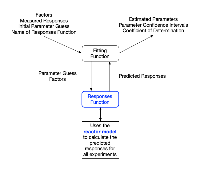
The flow of information to and from a numerically fitting function during the analysis of kinetics data is shown in Figure L.1. The fitting function calls the predicted responses function eqch time it needs to calculate the sum of the squares of the errors. Assuming the fitting function converges, it returns the best estimate for each rate expression parameter, the coefficient of determination, and the undertainty for each estimated parameter.
L.4 Assessment Graphs
For either a linear model or a numerical model, the fitting function returns the best estimates for the parameters, the coefficient of determination, and the undertainty in each estimated paramter. As described below, this information can be used to assess the accuracy of the fitted model. Additional insight into the accuracy of the fitted model can be gleaned from assessment graphs.
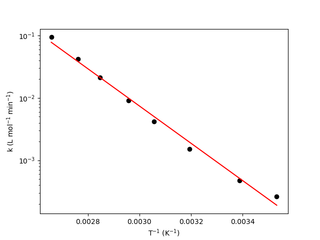
For linear models of the form of Equation L.1, a model plot is useful. In a model plot, Equation L.1 is plotted as a line, and \(\underline{y}_{expt}\) is plotted vs. \(x\) as points. When the model is the linearized form of the Arrhenius expression, the model plot can also be called and Arrhenius plot. Figure 4.5 from Example 4.5.4, reproduced here as Figure L.2, is an example of an Arrhenius plot. The red line shows the model-predicted rate coefficient as a function of reciprocal temperature, and the black circles show the experimentally measured rate coefficients as a function of reciprocal temperature.
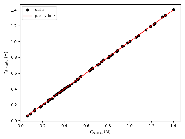
Two different kinds of graphs are helpful when assessing the accuracy of a numerical model. The first is callea a parity plot. In a parity plot the model-predicted responses are plotted versus the experimental responses as data points. The parity line, \(y_{expt} = y_{model}\), is then added to the graph. Figure 19.5, reproduced here as Figure L.3, is an example of a parity plot. The parity line representing points where the predicted and experimental responses are equal is shown in red and the data are shown as black circles. In that example, the final concentration of A, \(C_{A,f}\) was the response variable.
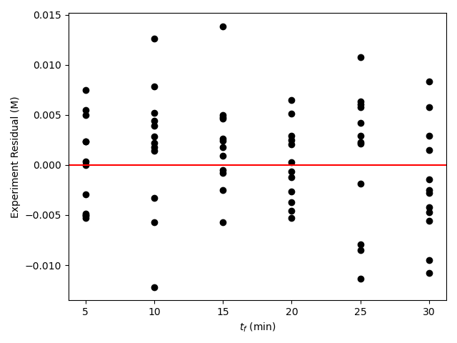
The second type of graph used with numerical models is called a residuals plot. The experiment residuals are the differences between the experimental responses and the model-predicted responses for the set of experiments, Equation L.13. A set of residuals plots can be created wherein the residuals are plotted versus each of the experimental adjusted input variables. Figure 19.6 includes the residuals plot shown in Figure L.4. It is an example of a residuals plot where the response variable was the final concentration of F and one of the adjusted inputs was the time at which the final concentration was measured. In the parity plot the experiment residuals are plotted as black circles and the horizontal axis where the residuals equal zero is shown in red.
\[ \epsilon_{expt,i} = y_{i,expt} - y_{i,model} \tag{L.13}\]
L.5 Assessing Model Accuracy
There are several indicators that a fitted model accurately represents the data to which it was fit. First, the coefficient of determination, \(R^2\), will be close to 1. The uncertainty in most of the estimated parameters, if not all, will be small relative to the extimated value. That is, the standard error for the parameter will be small compated to the value of the parameter or the upper and lower limits of the 95% confidence interval will be close to the estimated value of the parameter.
As noted in Chapter 18, there could be a few paramters for which the uncertainty is large but the model is still accurate. This could indicate one of three possibilities. First, the factor levels (values to which the adjusted input variables were set) used in the experiments may not allow accurate resolution of those parameters that have high uncertainty. Second, parameters with higher uncertainty may be mathematically coupled to each other (e. g. the model-predicted response may only depend on the product of two parameters so that the individual parameters can have any values as long as their product has the optimum value). Third, the parameters with high uncertainty may not be needed, and there may be a simpler model with fewer parameters that is equally accurate.
If there were no random errors in the experimental data and the model was exact, then every experimental data point in a model plot would fall on the line representing the model. If the model is accurate, the deviations of the data from the line will be small and random. There will not be any systematic trends in the deviations.
If there were no random errors in the experimental data and the model was exact, then every experimental data point in a parity plot would fall on the parity line, and every experiment residual would equal zero and fall on the horizontal axis. If the model is accurate, the deviations from data from the parity line will be small, and there will be no systematics trends in the deviations of the experiment residuals from the horizontal axis. If there are trends in the deviations of the experiment residuals, it may indicate that the model does not fully capture the effect of the plotted experimental input upon the response.
In Reaction Engineering Basics experiment residuals are only plotted against each of the adjusted inputs. However, a residuals plot can be generated for any aspect of the experiments that might affect the results of an experiment. For example the experiment residuals could be plotted against the technician who performed the experiment or against the vendor from whom a reagent was purchased.
Ultimately, deciding whether the model is sufficiently accurate is a judgement call. To summarize, the following criteria are satisfied by an accurate model.
- The coefficient of determination, \(R^2\), is nearly equal to 1.
- The uncertainty in most, if not all, of model parameters is small compared to the parameter’s value.
- When using standard errors of the parameters, they are small compared to the parameter value.
- When using 95% confidence intervals, the upper and lower limits of the interval are close to the parameter value.
- The points in the parity plot are all close to a diagonal line passing through the origin.
- In each residuals plot, the points scatter randomly about the horizontal axis, and no systematic deviations are apparent.
L.6 Mathematical Formulation of Parameter Estimation Calculations
In Reaction Engineering Basics, with only a few exceptions, parameter estimation will involve using a numerical fitting function to fit a predicted responses function to experimental data, and within the predicted responses function the reactor design equations for the experimental reactor will be solved numerically. A convenient way to mathematically formulate the calculations is to sequentially formulate the reactor model, the predicted responses function, the use of a numerical fitting function, and the generation of assessment graphs. Then the calculations can be succinctly summarized in terms of those components.
The reactor model should be formulated as described in Chapter 7. The rate expression parameters and the adjusted experimental inputs for one experiment should be shown as required input.
The formulation of the predicted responses function should list the arguments provided to it (the rate expression parameters and the adjusted experimental inputs for all experiments) and the values it returns (the model predicted responses for all experiments). It should provide the algorithm it uses, noting that for each expeirment it uses the reactor model to solve the design equations and then the results to calculate the model-predicted response.
The use of a numerical fitting function to estimate the rate expression parameters and statistics should be described including making an initial guess for the rate expression parameters, identifying the arguments that will be passed to the fitting function, identifying quantities that will be returned by the fitting function, and describing any final calculations that must be performed on the returned values.
Finally, the generation of assessment graphs should be described, noting what will be plotted and how the plotted quantities will be calculated.
L.7 Example
The following example illustrates the mathematical formulation of the estimation of rate expression parameters as described above.
L.7.1 Formulation of the Estimation of Rate Expression Parameters Using BSTR Data
A reaction engineer conducted kinetics experiments using an isothermal BSTR. The adjusted experimental inputs consisted of the temperature, the initial concentration of reagent A and the final time and the response was the fina concentration of reagent A. The proposed rate expression is shown in equation (1) where \(k_0\) and \(E\) are rate expression parameters. The engineer generated the following BSTR model.
Design Equations
\[ \frac{dn_A}{dt} = -rV \tag{3} \]
\[ \frac{dn_Z}{dt} = rV \tag{4} \]
Initial Values and Stopping Criterion
| Variable | Initial Value | Stopping Criterion |
|---|---|---|
| \(t\) | \(0\) | \(t_f\) |
| \(n_A\) | \(n_{A,0}\) | |
| \(n_Z\) | \(0\) |
Required Input: \(k_0\),, \(E\), \(C_{A,0}\), \(T\), and \(t_f\)
Derivatives Function
\(\qquad\) Arguments: \(t\), \(n_A\), and \(n_Z\)
\(\qquad\) Return values: \(\frac{dn_A}{dt}\), and \(\frac{dn_Z}{dt}\)
\(\qquad\) Algorithm:
\(\qquad \qquad\) 1. Evaluate the unknowns in equations (3) and (4).
\[ k = k_0\exp{\left( \frac{-E}{RT}\right)} \tag{5} \]
\[ C_A = \frac{n_A}{V} \tag{6} \]
\[ r = kC_A \tag{2} \]
\(\qquad \qquad\) 2. Evaluate the derivatives using equations (3) and (4).
\[ C_A = \frac{n_A}{V} \tag{5} \]
\[ r = kC_A \tag{2} \]
Solving the Design Equations
- Calculate unknown initial and final values.
\[ n_{A,0} = C_{A,0}V \tag{7} \]
Call an IVODE solver passing the initial values, stopping criterion and name of the derivatives function as arguments.
Receive and return corresponding sets of values of \(t\), \(n_A\), and \(n_B\) that span the range from the start of the experiment to the time when the response was measured.
Formulate the estimation of the rate expression parameters using this model.
Arguments: \(\underline{T}\), \(\underline{C}_{A,0}\), \(\underline{t}_{f}\), \(k_0\), and \(E\).
Return values: \(\underline{C}_{A,f}\)
Algorithm:
- Loop through the experiments, and for each experiment
- Make the adjusted experimental inputs for the experiment and the values of the rate expression parameters available to the BSTR model.
- Use the BSTR model to solve the design equations for \(\underline{t}\), \(\underline{n}_A\), and \(\underline{n}_Z\).
- Calculate and save the predicted response.
\[ C_{A,f,model} = \frac{n_A\big\vert_{t=t_f}}{V} \tag{8} \]
- Return the set of model-predicted responses.
- Set an initial guess for \(k_0\) and \(E\).
- Call a numerical fitting function
- passing the adjusted experimental inputs, \(\underline{T}\), \(\underline{C}_{A,0}\), and \(\underline{t}_{f}\), the experimental responses, \(\underline{C}_{A,f}\), the initial guess for the parameters, and the predicted responses function, above, as arguments
- receiving the parameter estimates, \(k_0\) and \(E\), the upper and lower limits of the 95% confidence interval for each parameter estimate, \(k_{0,CI,l}\), \(k_{0,CI,u}\), ,\(E_{CI,l}\) and \(E_{CI,u}\), and the coefficient of determination, \(R^2\).
- Calculate the model-predicted responses using the parameter estimates by calling the predicted responses function.
- Calculate the experiment residuals.
\[ \epsilon_{expt} = C_{A,f} - C_{A,f,model} \tag{9} \]
- Generate a parity plot showing \(\underline{C}_{A,f,expt}\) vs. \(\underline{C}_{A,f,model}\).
- Generate residuals plots showing \(\underline{\epsilon}_{expt}\) vs. \(\underline{T}\), vs. \(\underline{C}_{A,0}\), and vs. \(\underline{t}_{f}\).
L.8 Symbols Used in Appendix L
| Symbol | Meaning |
|---|---|
| \(b\) | intercept of a linear function. |
| \(j\) | Subscript indexing the reactions taking place. |
| \(k\) | Rate coefficient, a subscript is used to index the reactions if more than one are occurring. |
| \(k_{0}\) | Pre-exponential factor for a rate coefficient, an additional subscript is used to index the reactions if more than one are occurring. |
| \(m\) | Slope in a linear function, subscripts index the slopes when there are more than one. |
| \(n_i\) | Molar amount of reagent \(i\), an additional subscripted \(0\) denotes the initial molar amount. |
| \(r\) | Reaction rate. |
| \(t\) | Elapsed time, an additional subscripted \(f\) denotes the final time. |
| \(x\) | Adjusted input variable, a subscript denotes the experiment or the input. |
| \(y\) | Response, additional subscripts denote the experiment and whether the response was measured (expt) or predicted (model). |
| \(\hat{y}\) | Model-predicted response, a subscript is used to index the responses in an experimental data set. |
| \(C_i\) | Concentration of reagent \(i\), an additional subscripted \(0\) denotes the initial concentration, an additional subscripted \(f\) denotes the final concentration. |
| \(CI\) | 95% confidence interval; when used as a subscript followed by “u” or “l” it indicates that the current variable is an upper or lower 95% confidence interval limit. |
| \(E\) | Activation energy, a subscript is used to index the reactions if more than one are occurring. |
| \(N\) | Number of experiments in a data set. |
| \(R\) | Ideal gas constant. |
| \(R^2\) | Coefficient of determination. |
| \(T\) | Temperature. |
| \(V\) | Volume. |
| \(\lambda\) | Standard error in a parameter estimate, an additional subscript denotes the specific parameter. |
| \(\beta\) | Base-10 log of a pre-exponential factor when used as a rate expression parameter in place of the actual pre-exponential factor. |
| \(\epsilon_{expt}\) | Experiment residual; a subscript denotes the experiment. |
| \(\Psi\) | Sum of the squares of the errors or the relative errors between the experimental response and the model-predicted response. |
| \(\underline{ }\) | an underlined symbol denotes a set (or vector) of values. |