Appendix K — Solving Differential-Algebraic Equations
A set of differential-algebraic equations (DAEs) includes two subsets of equations. One subset contains IVODEs and the other contains ATEs. The distinguishing feature of DAEs is that the IVODEs and the ATEs are coupled. That is, there are some unknowns that appear in both the IVODEs and the ATEs. In Reaction Engineering Basics, DAEs are only encountered when analyzing simple reactor systems that include a PFR.
When a set of ATEs is solved numerically, a computer program called an ATE solver is used. Appendix I describes how ATE solvers work, what they require as input, and how to use them. Similarly, when a set of IVODEs is solved numerically an IVODE solver is used. Appendix J describes how IVODE solvers work, what they require as input, and how to use them.
When a set of DAEs of the kind encountered in Reaction Engineering Basics needs to be solved, it isn’t necessary to use a DAE solver. The DAEs can be solved using ATE and IVODE solvers. Thus, assuming the reader is familiar with Appendices I and J, this appendix does not need to describe how a DAE solver works, what it requires as input, or how to use it. However, in order to solve the DAEs using ATE and IVODE solvers, the equations need to be formulated properly. The purpose of this appendix, then, is to describe how to mathematically formulate the solution of a set of DAEs so that they can be solved using ATE and IVODE solvers.
K.1 DAEs in Reaction Engineering Basics
In Reaction Engineering Basics the IVODE subset of the DAEs will always be the reactor design equations for a PFR. The ATE subset of the DAEs will be mole and energy balances on other equipment connected to the PFR. Specifically the ATEs will be mole and energy balances on a heat exchanger when analyzing a thermally back-mixed PFR or mole and energy balances on a stream mixer when analyzing a recycle PFR.
Appendix J describes how to solve IVODEs with an unknown initial value or when an unknown constant appears in the IVODEs. In essence, an implicit ATE is written for the unknown initial value or constant. The IVODEs then are solved each time the residual for the implicit ATE is evaluated. The solution of a set of DAEs as described here uses a very similar approach.
K.2 Mathematical Formulation of the Solution of DAEs
After summarizing the assignment, the mathematical formulation of the solution should begin with the formulation of a model for the PFR only. Doing so will reveal whether the PFR design equations can be solved independently from the equations for all other equipment in the system. If they can, then the IVODEs are not mathematically coupled to any ATEs, and the information in this appendix is not needed. In many cases, however, formulating the PFR design equations will show that they cannot be solved independently. Specifically, the necessary initial values of one or more dependent variables will be unknown.
If the IVODEs cannot be solved independently, the next step is to formulate a model for the heat exchanger or stream mixer that precedes the PFR in the system. Formulation of this model will reveal that there are more unknowns than equations. If the equations in this model were going to be solved analytically, this would mean that they could not be solved independently. In essence, in order to solve the PFR model, the solution of the heat exchanger or mixer model would be needed, and to solve the heat exchanger or mixer model, the solution to the PFR design equations would be needed.
When the heat exchanger or stream mixer model (ATEs) is going to be solved numerically, however, that is not the case. As noted, the number of unknown quantities will be greater than the number of ATEs. The unknown quantities appearing in the ATEs will include the initial values of the IVODE dependent variables, among other unknown quantities. The key to solving the ATEs is to include the unknowns that are also initial values in the IVODEs among the unknowns to be found by solving the ATEs.
As described in Appendix I, when an ATE solver is used to solve the ATEs numerically, it must be provided with two things. The first is an initial guess for the solution of the ATEs. The second is a residuals function. The residuals function must accept a guess for the solution of the ATEs as an argument. It must use that guess to calculate the values of any remaining unknown quantities appearing in the residuals expressions, evaluate the residuals, and return their values.
So in the present situation, the ATEs are being solved to find the IVODE initial values (and perhaps other quantities). As such, when the residuals function will receive a guess that includes the IVODE initial values. Using those initial values, the IVODEs can be solved numerically within the residuals function. The results from doing so can then be used to calculate any additional unknown quantities appearing in the residuals expressions, after which, the residuals can be evaluated.
The key point is that the IVODEs are solved numerically within the residuals function where the necessary initial values are available. The numerical solution of the IVODEs can be accomplished exactly as described in Appendix J.
K.3 Numerical Implementation of the Solution of DAEs
The mathematical formulation of the solution began with the formulation of a PFR model wherein the PFR reactor design equations are solved. The numerical implementation of the solution begins with writing related computer functions. Specifically, a PFR model function and a derivatives function must be written as detailed here.
- derivatives function
- receives the values of the independent and dependent variables at the start of an integration step as arguments, uses them to evaluate the derivatives and returns their values.
- PFR model function
- receives the initial values of the dependent variables as arguments, calls an IVODE solver, passing the initial values, stopping criterion, and the name of the derivatives function above, checks that a solution was obtained, and returns corresponding sets of values of the independent variable and each of the dependent variables spanning the range from the reactor inlet to the reactor outlet.
The next step in the mathematical formulation was the formulation of a model for the heat exchanger or stream mixer. The next step in the numerical implementation is writing related computer functions. The heat exchanger/stream mixer model is a set of ATEs, so a heat exchanger/stream mixer model function that solves those ATEs and a residuals function must be written as described here.
- residuals function
- receives a guess for the solution of the ATEs that includes the initial values needed to solve the PFR design equations, calls the reactor model function, passing those initial values as argument, to solve the IVODEs, uses the results to calculate any other unknown quantities appearing in the ATEs, evaluates the residuals and returns their values.
- heat exchanger/stream mixer model function
- receives an initial guess for the solution of the heat exchanger/stream mixer design equations (i. e. the ATEs), calls an ATE solver, passing the initial guess and the name of the residuals function above as arguments, checks that the ATE solver converged, and returns one solution of the ATEs.
The numerical implementation is completed by writing an analysis function that uses the preceding functions to perform the analysis and calculate the quantities of interest
- analysis function
- establishes a mechanism for making quantities available to all functions, sets an initial guess for the solution of the other equipment ATEs, calls the other equipment model function to get a solution of the ATEs, and perfroms any additional calculations that are necessary.
K.4 Example
This appendix did not introduce any new numerical methods. The one new topic it touched on was how to structure the solution mathematically so that the analysis can be performed using ATE and IVODE solvers. As such, there aren’t any new numerical methods that need to be demonstrated, and it isn’t clear that an example is necessary. As a compromise, Example 17.3.1 is reproduced here, but with different expert thinking callouts that are intended to highlight how the solution of the ATEs was formulated to allow solution of the models. The equations used in the example are not derived here, see Example 17.3.1 for that.
K.4.1 Numerical Aspects of Modeling a Recycle PFR
In liquid phase reaction (1) the chiral molecule, Z, is produced auto-catalytically according to the rate expression given in equation (2). In the absence of the product, Z, the reaction rate is very small. The heat of reaction is -14 kcal mol-1, independent of temperature. The pre-exponential factor is equal to 4.2 x 1015 cm3 mol-1 min-1 and the activation energy is 18 kcal mol-1. A solvent is used, and the heat capacity of the reacting solution can be taken to equal that of the solvent, 1.3 cal cm-3 K-1. The density of the liquid may be assumed to be constant. The concentrations of A and Z in the feed to the process are 2 M and 0 M, respectively, and the flow rate is 500 cm3 min-1 at 300K. An adiabatic recycle PFR with a recycle ratio of 1.3 is used. The reactor diameter is 5 cm and it is 50 cm long. What are the outlet concentrations of A and Z and the outlet temperature from the process?
\[ A \rightarrow Z \tag{1} \]
\[ r_1 = k_1C_AC_Z \tag{2} \]
K.4.1.1 Assignment Summary
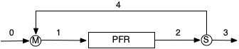
System Schematic
Reactor Type: Adiabatic PFR
Quantities of Interest: \(C_{A,3}\), \(C_{Z,3}\), and \(T_3\)
Given and Known Constants: \(\Delta H_1\) = -14 kcal mol-1, \(k_{0,1}\) = 4.2 x 1015 cm3 mol-1 min-1, \(E_1\) = 18 kcal mol-1, \(\breve{C}_p\) = 1.3 cal cm-3 K-1, \(C_{A,0}\) = 2 M, \(C_{Z,0}\) = 0 M, \(\dot{V}_0\) = 500 cm3 min-1, \(T_0\) = 300K, \(R_R\) = 1.3, \(D\) = 5 cm, \(L\) = 50 cm, and \(R\) = 1.987 cal mol-1 K-1.
K.4.1.2 Mathematical Formulation of the Solution
PFR Model
Design Equations
\[ \frac{d \dot{n}_{A,PFR}}{d z} = - \frac{\pi D^2}{4}r_1 \tag{3} \]
\[ \frac{d \dot{n}_{Z,PFR}}{d z} = \frac{\pi D^2}{4}r_1 \tag{4} \]
\[ \frac{dT_{PFR}}{dz} = - \frac{\pi D^2}{4} \frac{r_1 \Delta H_1}{\dot{V}_{PFR} \breve{C}_p} \tag{5} \]
Initial Values and Stopping Criterion
| Variable | Initial Value | Stopping Criterion |
|---|---|---|
| \(z\) | \(0\) | \(L\) |
| \(\dot{n}_{A,PFR}\) | \(\dot{n}_{A,1}\) | |
| \(\dot{n}_{Z,PFR}\) | \(\dot{n}_{Z,1}\) | |
| \(T_{PFR}\) | \(T_1\) |
Derivatives Function
Given the values of \(z\), \(\dot{n}_{A,PFR}\), \(\dot{n}_{Z,PFR}\), and \(T_{PFR}\) and those listed in the assignment summary, the unknown quantities appearing in equations (3) through (5) can be evaluated using the following sequence of calculations. The derivatives can then be evaluated using equations (3) through (5).
\[ \dot{V}_3 = \dot{V}_0 \]
\[ \dot{V}_4 = R_R \dot{V}_3 \]
\[ \dot{V}_2 = \dot{V}_3 + \dot{V}_4 \]
\[ \dot{V}_{PFR} = \dot{V}_2 \]
\[ k_1 = k_{0,1} \exp \left( \frac{-E_1}{RT} \right) \]
\[ C_A = \frac{\dot{n}_A}{\dot{V}} \]
\[ C_Z = \frac{\dot{n}_Z}{\dot{V}} \]
\[ r_1 = k_1 C_A C_Z \]
Solving the PFR Design Equations
I cannot solve the PFR reactor model because I do not know the initial values, \(\dot{n}_{A,1}\), \(\dot{n}_{Z,1}\), and \(T_1\). I need equations for calculating those values, so I’ll write mole and energy balances on the stream mixer, M.
Stream Mixer Model
Design Equations
\[ 0 = \dot{n}_{A,1} - \dot{n}_{A,0} - \dot{n}_{A,4} = \epsilon_1 \tag{6|} \]
\[ 0 = \dot{n}_{Z,1} - \dot{n}_{Z,0} - \dot{n}_{Z,4} = \epsilon_2 \tag{7} \]
\[ 0 = \dot{V}_0 \breve{C}_p \left( T_1 - T_0 \right) + \dot{V}_4\breve{C}_p \left( T_1 - T_4 \right) = \epsilon_3 \tag{8} \]
These three ATEs contain nine unknowns. Three of them, \(\dot{n}_{A,1}\), \(\dot{n}_{Z,1}\), and \(T_1\), are the initial values I need in order to solve the PFR reactor model equations. The others are \(\dot{n}_{A,0}\), \(\dot{n}_{Z,0}\), \(\dot{n}_{A,4}\), \(\dot{n}_{Z,4}\), \(\dot{V}_4\), and \(T_4\). I can easily calculate \(\dot{n}_{A,0}\), \(\dot{n}_{Z,0}\), and \(\dot{V}_4\).
\[ \dot{n}_{A,0} = \dot{V}_0 C_{A,0} \]
\[ \dot{n}_{Z,0} = \dot{V}_0 C_{Z,0} \]
\[ \dot{V}_3 = \dot{V}_0 \]
\[ \dot{V}_4 = R_R \dot{V}_3 \]
That leaves me with three ATEs containing six unknowns: \(\dot{n}_{A,1}\), \(\dot{n}_{Z,1}\), \(T_1\), \(\dot{n}_{A,4}\), \(\dot{n}_{Z,4}\), and \(T_4\). I know that in this situation, the key is to include the initial values for the IVODEs among the unknowns to be found by solving the ATEs. In this example there are only three ATEs, so they can be solved to find the three unknown initial values, \(\dot{n}_{A,1}\), \(\dot{n}_{Z,1}\), and \(T_1\).
Residuals Function
Equations (6) through (8) will be solved for \(\dot{n}_{A,1}\), \(\dot{n}_{Z,1}\), and \(T_1\). The residuals must be evaluated given a guess for those quantities. Using that guess and the values listed in the assignment summary, the PFR model equations can be solved for \(\dot{n}_{A,PFR}\), \(\dot{n}_{Z,PFR}\), and \(T_{PFR}\). Then the following sequence of calculations can be used to find \(\dot{n}_{A,4}\), \(\dot{n}_{Z,4}\), and \(T_4\).
\[ \dot{n}_{A,2} = \dot{n}_{A,PFR} \big \vert_{z=L} \]
\[ \dot{n}_{Z,2} = \dot{n}_{Z,PFR} \big \vert_{z=L} \]
\[ T_4 = T_3 = T_2 = T_{PFR} \big \vert_{z=L} \]
\[ \dot{n}_{A,4} = \frac{R_R}{1 + R_R}\dot{n}_{A,2} \]
\[ \dot{n}_{Z,4} = \frac{R_R}{1 + R_R}\dot{n}_{Z,2} \]
The residuals, \(\epsilon_1\), \(\epsilon_2\), and \(\epsilon_3\), can then be evaluated using equations (6) through (8).
Solving the Stream Mixer Design Equations
The stream mixer design equations can be solved by calling an ATE solver, providing it with the initial guess for \(\dot{n}_{A,1}\), \(\dot{n}_{Z,1}\), and \(T_1\) and a function that evaluates the residuals as described above. The results returned by the solver should be checked to make sure the solver converged. Assuming it did converge, it will return the values of \(\dot{n}_{A,1}\), \(\dot{n}_{Z,1}\), and \(T_1\).
Performing the Analysis
The complete analysis can be performed as follows.
- Guess the values of \(\dot{n}_{A,1}\), \(\dot{n}_{Z,1}\), and \(T_1\).
- Use the stream splitter model as described above to calculate \(\dot{n}_{A,1}\), \(\dot{n}_{Z,1}\), and \(T_1\).
- Provide the results to the PFR model and use it as described above to get corresponding sets of values of \(z\), \(\dot{n}_{A,PFR}\), \(\dot{n}_{Z,PFR}\), and \(T_{PFR}\) that span the range from the reactor inlet to the reactor outlet.
- Perform the following sequence of calculations to find the quantities of interest, \(C_{A,3}\), \(C_{Z,3}\), and \(T_3\).
\[ \dot{n}_{A,2} = \dot{n}_{A,PFR} \big \vert_{z=L} \]
\[ \dot{n}_{Z,2} = \dot{n}_{Z,PFR} \big \vert_{z=L} \]
\[ T_4 = T_{PFR} \big \vert_{z=L} \]
\[ \dot{n}_{A,4} = \frac{R_R}{1 + R_R}\dot{n}_{A,2} \]
\[ \dot{n}_{Z,4} = \frac{R_R}{1 + R_R}\dot{n}_{Z,2} \]
\[ \dot{n}_{A,3} = \dot{n}_{A,2} - \dot{n}_{A4} \]
\[ \dot{n}_{Z,3} = \dot{n}_{Z,2} - \dot{n}_{Z4} \]
\[ \dot{V}_3 = \dot{V}_0 \]
\[ C_{A,3} = \frac{\dot{n}_{A,3}}{\dot{V}_3} \]
\[ C_{Z,3} = \frac{\dot{n}_{Z,3}}{\dot{V}_3} \]
K.4.1.3 Numerical implementation of the Solution
Create a computer function and within that function do the following:
- Make the given and known constants available everywhere within the function.
- Write a derivatives function that
- receives the independent and dependent variables, \(z\), \(\dot{n}_A\), \(\dot{n}_Z\), and \(T\), as arguments,
- evaluates the derivatives as described above for the PFR model, and
- returns the values of \(\frac{d\dot{n}_{A,PFR}}{dz}\), \(\frac{d\dot{n}_{Z,PFR}}{dz}\), and \(\frac{dT_{PFR}}{dz}\).
- Write a PFR function that
- \(\dot{n}_{A,1}\), \(\dot{n}_{Z,1}\), and \(T_1\) as arguments,
- solves the PFR reactor design equations as described above for the PFR model, and
- returns corresponding sets of values of \(z\), \(\dot{n}_{A,PFR}\), \(\dot{n}_{Z,PFR}\), and \(T_{PFR}\).
- Write a residuals function that
- receives \(\dot{n}_{A,1}\), \(\dot{n}_{Z,1}\), and \(T_1\) as arguments,
- evaluates the residuals as described above for the stream mixer model, and
- returns the values of \(\epsilon_1\), \(\epsilon_2\), and \(\epsilon_3\).
- Write a stream mixer model function that
- receives guesses for \(\dot{n}_{A,1}\), \(\dot{n}_{Z,1}\), and \(T_1\) as arguments,
- calculates \(\dot{n}_{A,1}\), \(\dot{n}_{Z,1}\), and \(T_1\) as described above for the stream mixer model, and
- returns the resulting values of \(\dot{n}_{A,1}\), \(\dot{n}_{Z,1}\), and \(T_1\).
- Write an analysis function that performs the analysis as described above and displays the results.
- Call the analysis function.
K.5 Symbols Used in Appendix K
| Symbol | Meaning |
|---|---|
| \(k_0\) | Arrhenius pre-exponential factor; an additional subscript indexes the reaction. |
| \(\dot{n}\) | Molar flow rate; additional subscripts denote the reagent and identify the flow stream. |
| \(r\) | Reaction rate; additional subscripts index the reaction. |
| \(z\) | Axial distance from the inlet of a PFR. |
| \(\breve{C}_p\) | Volumetric heat capacity. |
| \(D\) | PFR diameter. |
| \(E\) | Activation energy; an additional subscript indexes the reaction. |
| \(L\) | Length of a PFR. |
| \(P\) | Pressure. |
| \(R\) | Ideal gas constant. |
| \(R_R\) | Recycle ratio. |
| \(T\) | Temperature; an additional subscript denotes the flow stream. |
| \(\dot{V}\) | Volumetric flow rate; an additional subscript denotes the flow stream. |
| \(\Delta H\) | Heat of reaction; an additional subscript indexes the reaction. |